Basics of Tool Design--Inspection and Gage Design

Tolerance

A drawing of a workpiece may be used as a guide for its manufacture only if it completely defines its limits of size, shape, and composition with dimensions and specifications. Tolerances may be given (directly or indirectly) for every dimension or specification.

Tolerance is the total amount by which a dimension may vary from a specified size. When providing tolerances, the designer recognizes that no two workpieces, distances, or quantities can be exactly alike. The designer specifies an ideal condition (nominal dimension), then states what degree of error can be tolerated.

Each dimension on a workpiece must be specified as being between two limits. No proper dimension can ever be given as a single fixed value because a single value is unrealistic in traditional manufacturing. The designer guards against this pitfall in several ways. Critical dimensions on a drawing have the tolerance given as part of the dimension (for example, .125 ±.002 in. [3.18 ±0.05 mm]). Less critical dimensions are provided tolerance by a general note in the title block (for example, unless otherwise specified, all dimensions are ±.010 in. [±0.25 mm]). Tolerance also may be specified indirectly in the bill of material. If the designer calls for the use of purchased material or parts and does not further specify tolerance, it must be assumed that the vendor's manufacturing tolerances are acceptable.

When establishing tolerances, the designer may consider a number of factors, including function, appearance, and cost. The workpiece will have an intended function, and the specified tolerance must be compatible with it. Appearance is sometimes a factor because a workpiece dimension with no actual function may have aesthetic requirements (among others). If for no other reason than the cost of materials, the size of a workpiece must be limited.

Cost can be the governing factor when deciding tolerances. As tolerances become tighter, the cost of meeting them rapidly increases. The designer, in concert with other departments, often must weigh the need for a close tolerance against its cost, along with the capability of the machines that will produce the workpiece. If the function of the workpiece requires extremely close tolerances to ensure proper mating allowances, it may be less expensive to combine easily held tolerances with selective assembly. It may be possible in this way to obtain the necessary mating allowances for the specific function without increasing the cost with close tolerances.

In a conventional drawing, the workpiece is shown in a fixed relationship to Reference planes at right angles to each other. The location of each element of the workpiece is defined by stating its distance (dimension) from each Reference plane. Each dimension has a tolerance.

The Reference planes in a single view may be compared with the X and Y axes of the Cartesian coordinate system. The location of the element is anywhere within a rectangular area formed by the minimum and maximum values of the X and Y dimensions as established by the tolerances.

Engineering intent often can be expressed more exactly by stating the nominal location of the element and how far from the true position (TP) the element may vary. In this case, a positional tolerance applied to the nominal location takes the place of the X and Y tolerances as shown in FIG. 1. The workpiece designer's intent can be further shown by modern geometric dimensioning and tolerancing methods (see Section 13).

Conversion charts

Since most machine movements are made in two directions at 90° to one another, X and Y, the chart shown in FIG. 2 may be used to deter mine the two-sided tolerance approximations of positional tolerance diameters. Mathematically, they also can be approximated by multiplying the position tolerance, ?, by 0.7.

For example, 0.7 × 0.010 = 0.0070 ÷ 2 in. = ±.00350 in. (0.7 × 0.35 = 0.245 ÷ 2 = ±0.1225 mm).

The chart in FIG. 3 may be used to deter mine whether an actual hole center (as measured on an open setup) is within the positional tolerance specified on the drawing, and the actual amount of difference (radius) from TP. For example, on a drawing, a hole is located by dimensions labeled TP with a positional tolerance. The location of the actual center of the hole on the part is determined by coordinate measurements. The difference in the actual measurements and corresponding TP dimensions are located on the chart using the values in the upper and right-hand borders. It can then be shown whether the location is within the required positional tolerance limits using values in the left-hand border.

To determine the actual difference from TP, a radius may be drawn through the point, intersecting the 45° diagonal line. The amount of difference may now be read from the scale on the 45° line using the values in the lower border.

Mathematically, it also can be approximated by multiplying the total ± tolerance by 1.4. For example, 1.4 × .007 in. = .010 in. (±.0035 in.) (1.4 × 0.20 mm = 0.28 mm [±0.100 mm]).

Gaging principles

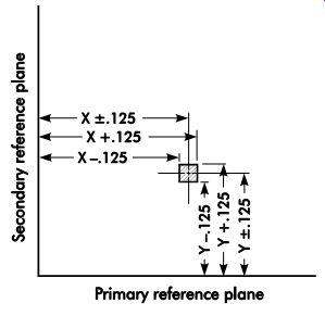
FIG. 1. Coordinate dimensioning and positioning tolerance illustrate the element. The dimension may be located anywhere within the shaded rectangle.

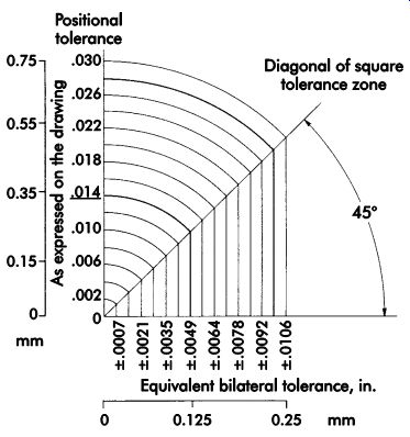
FIG. 2. Conversion chart: positional tolerance to bilateral.

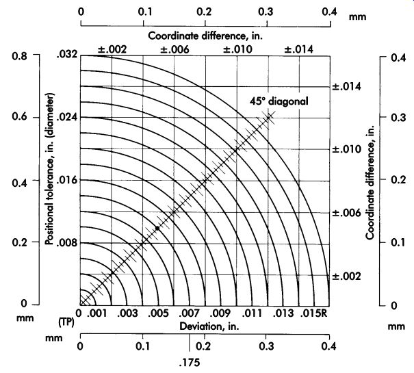
FIG. 3. Conversion chart: bilateral to positional tolerance.

Since it is not feasible to produce many parts with exactly the same dimensions, working tolerances are necessary. For the same reason, gage tolerances are necessary. Gage tolerance is generally determined from the amount of workpiece tolerance. For fixed, limit-type working gages, the 10% rule is typically used to determine the amount of gage tolerance. Thus, in the absence of a specified gage tolerance, the gagemaker will use 10% of the workpiece tolerance as the gage tolerance for a working gage. Working gages are those used by production workers during manufacturing.

The amount of tolerance on inspection gages-those used by the inspection department-is generally 5% of the workpiece tolerance. Tolerance on master gages-those used for checking the accuracy of other gages-is generally 10% of the gage tolerance. Where tolerances are large, gages used by the inspection department are not different from the working gages.

Four classes of gagemakers' tolerances have been established by the American Gage De sign Committee and are in general use. These four classes establish maximum variations for any desired gage size. The degree of accuracy needed determines the class of gage to be used.

TBL. 1 shows the four classes of gagemakers' tolerances.

TBL. 1. Standard gagemakers' tolerances, in. (mm)

• Class XX gages are precision smoothed (lapped) to the very closest tolerances practicable. They are used primarily as master gages and for final close-tolerance inspection.

• Class X gages are precision lapped to close tolerances. They are used for some types of master gage work and as close-tolerance inspection and working gages.

• Class Y gages are precision lapped to slightly larger tolerances than Class X gages. They are used as inspection and working gages.

• Class Z gages are precision lapped. They are used as working gages where part tolerances are large and the number of pieces to be gaged is small.

Going from Class XX to Class Z, tolerances be come increasingly greater, and the gages are used for inspecting parts having increasingly larger work tolerances.

To show the use of the 10% rule in connection with TBL. 1, assume a gagemaker is to choose the correct tolerance class for a working plug gage to be used on a 1.0000-in. (25.400-mm) diameter hole having a working tolerance of .0012 in. (0.030 mm). One-tenth of the work tolerance would indicate a gage tolerance of .00012 in. (0.0031 mm), as noted in the table, a class Z gage. If the working tolerance were only .0006 in. (0.015 mm) on the 1.0000-in. (25.400-mm) diameter hole, then a class X gage would be indicated, with a tolerance of .00006 in. (0.0015 mm). If the working tolerance, however, were .015 in. (0.38 mm), then the gage tolerance indicated by the 10% rule would be .0015 in. (0.381 mm). As this is larger than the maxi mum tolerance class, a class Z gage would be needed, and the gage tolerance would be .00012 in. (0.0031 mm).

The smaller the degree to which a gage tolerance must be held, the more expensive the gage becomes. Just as production cost rises sharply as working tolerances are reduced, the cost of buying or manufacturing a gage is much higher if close tolerances are specified. Gage tolerances should be realistically applied using the work piece tolerance and the 10% rule.

Allocation of Gage Tolerances

After deciding the tolerance for a specific gage, the direction (plus or minus) of that allowance must be decided. Two basic systems-the bilateral and unilateral-and the many variations to them, are used when making this decision. The final results of these allocation systems will differ greatly. The choice of the system to be used, modified, or unmodified must be determined by the product and the facilities for producing it. The objectives when choosing an allowance system should be the economical production of as near to 100% usable parts as possible, and the acceptance of good pieces and rejection of bad.

The Bilateral System

In the bilateral system, the go and no-go gage tolerance zones are divided into two parts by the high and low limits of the workpiece's tolerance zone. The division is illustrated by FIG. 4a, which shows the gray rectangles representing the gage tolerance zones are half plus and half minus in relation to the high or low limit of the work tolerance zone.

In TBL. 1, assume that the diameter of the hole to be gaged is 1.2500 ±.0006 in. (31.750 ±0.015 mm). The total work tolerance in this case is .0012 in. (0.031 mm), since the hole size may vary from 1.2506 to 1.2494 in. (31.765 to 31.735 mm). Using 10% of the total work tolerance as the gage tolerance, the gage tolerance is then .00012 in. (0.0031 mm). From TBL. 1, this diameter would require a Class Z gage tolerance. The diameter on the go plug gage for this example would be 1.2494 ±.00006 in. (31.735 ±0.0015 mm), and the diameter of the no-go gage would be 1.2506 ±.00006 in. (31.765 ±0.0015 mm).

One disadvantage of the bilateral system is that parts not within the working limits can pass inspection. Using the previous example, if the hole to be gaged is reamed to the low limit (1.2494 in. [31.735 mm]) and if the go plug gage is at the low limit (1.24934 in. [31.7332 mm]), then the go plug gage will enter the hole and the part will pass inspection, even though the diameter of the hole is outside of the working tolerance zone. A part passed under these conditions would be very close to the working limit, and the tolerance on the mating part should not be such as to prevent assembly. Plug gages using the bilateral system also could pass parts in which the holes are too large. A common misconception is that gages accept good parts and reject bad. With the bilateral system, parts also can be rejected as being outside the working limits when they are not.

The Unilateral System

In the unilateral system (FIG. 4b), the work tolerance zone includes the gage tolerance zone. This makes the work tolerance smaller by the sum of the gage tolerance, but guarantees that every part passed by such a gage, regardless of the amount of the gage size variation, will be within the work tolerance zone.

If the diameter of the hole is 1.2500 ±.0006 in. (31.750 ±0.015 mm), again using 10% of the working tolerance as the gage tolerance, the go-gage diameter would be 1.24940 +.00012 in. (31.7348 +0.0031 mm), and the no-go gage diameter 1.25060 -.00012 in. (31.7652 -0.0031 mm).

The unilateral system of applying gage tolerance, like the bilateral system, may reject parts as being outside the working limits when they are not, but all parts passed using the unilateral system will be within the working limits. The unilateral system has found wider use in industry than the bilateral system for plain plug and ring gages.

One partial solution to the problem of gages rejecting parts that are within working limits is to use working gages with the largest unilateral gage tolerance practical, and inspection gages with the smallest unilateral gage tolerance practical. Thus, no piece can pass inspection that is outside of the tolerance, and the possibility of the inspection gage rejecting acceptable work is reduced because of its small tolerance.

FIG. 4c shows the commercial practice of allocating the plain ring gage tolerances negatively with Reference to both the maximum and minimum limits of the workpiece tolerance. In another practice (FIG. 4d), the no-go gage tolerance is divided by the maximum limit of the workpiece tolerance, and the go-gage tolerance is held within the minimum limit of the workpiece tolerance.

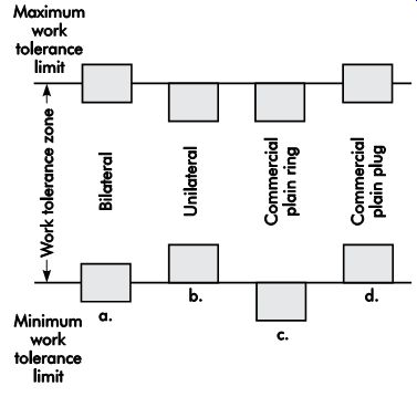
FIG. 4. Different systems of gage tolerance al location.

Gage Wear Allowance

Perfect gages cannot be made. If one did exist, it would no longer be perfect after just one checking operation. Although the amount of gage wear during just one operation is difficult to determine, it is easy to measure the total wear of several checking operations. A gage can wear beyond usefulness unless some allowance for wear is built into it.

The wear allowance is an amount added to the nominal diameter of a go plug and subtracted from that of a go ring gage. It is depleted during the gage's life by wearing away the gage metal.

Wear allowance is applied to the nominal gage diameter before the gage tolerance is applied.

The amount of wear allowance does not have to be decided in relation to work tolerance, al though a small work tolerance can restrict wear allowances. When specifying a wear allowance, the material from which the gage and work are to be made, the quantity of work, and the type of gaging operation to be performed must be taken into consideration. It is important to establish a specific amount of wear allowance. When the gage has worn the established amount, it should be removed from service without question. This avoids any controversy as to whether a gage is still accurate.

One method, which uses a percentage of the working tolerance as the wear tolerance, can be explained with the following example: For a 1.500 ±.0006 in. (38.10 ±0.015 mm) diameter hole, the working tolerance is .0012 in. (0.031 mm). The basic diameter of the go plug gage would be 1.49940 in. (38.0848 mm). Using 5% of the working tolerance (.00006 in. [0.0015 mm]) as the wear allowance, and adding this to the basic diameter, the new basic diameter then would be 1.49946 in. (38.0863 mm). The gagemaker's tolerance of 10% of the working tolerance (.00012 in. [0.0031 mm]) then would be applied in a plus direction as allowed by the unilateral system, with a resultant go plug diameter of 1.49946 (38.0863). Some manufacturing companies do not build a wear allowance into their gages, but create a standard to determine when a gage has worn beyond its usefulness. The gage is allowed to wear a certain percentage above or below its basic size before being taken out of service.

Gages should be inspected regularly for wear.

No set policy for wear allowance or gage inspection is practical for all industries. In operations where an extremely high degree of accuracy must be maintained, the amount of allowable wear is smaller, and inspection must be more frequent than in operations where tolerances are greater.

A gagemaker normally makes the gage to pro vide maximum wear, even if no wear allowance is designed into it. That is, the go end of a plug gage is made to its high limit, and the go component of a ring gage is made to its low limit.

The no-go gage will slip in or over very few pieces and wear very little. As any wear on a no go gage puts that gage farther within the product limits, no wear allowance is applied. Thus when the no-go gage begins to reject work within acceptable limits, it must be retired.

Gage Materials

For medium production runs, hardened alloy steel is used for the wear surfaces of gages. For higher-volume production runs, gage wear surfaces are usually chromium plated. When a high degree of accuracy is needed, the production run is long, and/or wear is excessive, tungsten-carbide contacts often are used on gages. Worn gaging surfaces can be ground down, chrome plated, reground, lapped to size, and put back into service.

Gaging policy

Gaging policy is the standardization of methods for determining gage tolerances, their allocation, and fixing wear allowance. It is a guide to determine when gages are required, when and how they are to be inspected, and the types to be used. Further, the policy addresses the conditions in which the gages will be used. Some production gaging is fine when performed near the machining operations. Other gaging will necessitate temperature, humidity, and vibration control.

There is no single policy in universal use. Gage users should have their own policy-the one best suited to their work. A gaging policy helps to eliminate controversy over the method of gaging, gage tolerances, allocation, and wear.

The policy establishes a general rule for deter mining the amount of gage tolerance. The 10% rule, used in conjunction with the four standard classes of gage tolerances, is widely used in industry.

The size and application of wear allowance is fixed in the gage policy. How often gages are inspected will depend upon how often they are used, the materials they check, and the closeness of tolerances. When a high degree of accuracy is needed, the gage policy must be strict.

Gage Measurement

A measurement compares an amount or length with a known standard. Dimensions are proven by end measurement. For example, the end of a specified length is measured against the end of the standard, just as the last drop of a specified amount of liquid brings a fluid level up to a mark on the side of the vessel. Almost all dimensional measurement is end measurement, which is determined by origin-both the standard and the length or amount being measured must start at a common point.

Every workpiece related to primary, secondary, and tertiary datums must be measured by three planes located at right angles to each other. Every dimension has as its origin one of the three planes. Given a horizontal Reference plane, two vertical Reference planes can be constructed at right angles to each other, and any structure can be defined by dimensions starting at the reference planes.

Surface plate

The surface plate is used as the main horizontal Reference plane. It is the primary tool of layout and inspection. Surface plates are usually made of cast iron or granite, with one surface finished extremely flat. When accuracy of .00001 in. (0.0003 mm) or finer is required, toolmakers' flats or optical flats are used instead. A number of accessories, such as squares, straight edges, parallels, angle irons, sine plates, leveling tables, height gages, length standards, and indicating equipment are used with the surface plate.

The workpiece being inspected is carefully placed with its primary Reference plane on the plate surface. If the workpiece has elements extending below its established Reference plane, it may be necessary to mount the workpiece on adjustable supports (jacks) or parallels to make the two reference planes parallel. Vertical Reference planes are placed on the surface plate as required.

To avoid an increased chance of error, all dimensions on a part drawing should start from a Reference point or plane rather than from the end of another dimension. If, however, a work piece feature is measured from a point rather than a Reference plane, its location should be proven in relation to that point rather than the Reference plane. A typical surface plate setup is shown in FIG. 5.

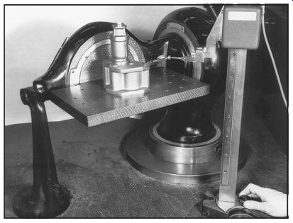
FIG. 5. Typical surface plate setup.

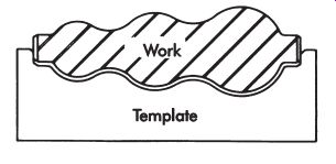
FIG. 6. Gaging the profile of a workpiece with a template.

Templates

A template represents a specified profile, or it may be a guide to the location of workpiece features with Reference to a single plane. A straightedge may be used as a template to check straightness.

To control or gage special shapes or contours in manufacturing, special templates are used for comparison by eye to ensure uniformity of individual parts. These templates are made from thin, easily machinable materials, some of which may be hardened later if production requirements demand longer use. FIG. 6 shows an application of the contour template to inspect a turned surface. Templates of this type are widely used in the sheet-metal industry, and where production is limited. They are satisfactory when the part tolerance will permit this type of inspection.

Gage Types

Commercial Gages

To inspect or gage radii or fillets visually, a standard commercial type of template can be obtained from various gage manufacturers.

These templates or gages are used by inspectors, layout personnel, toolmakers, diemakers, machinists, and pattern makers. The five different basic uses are shown in FIG. 7. These gages are usually made to nominal sizes in increments of 1/64 in. for inch gages (0.5 mm for millimeter gages). Special gages of this type may be readily designed and made for specific jobs.

Screw Pitch Gage

A screw pitch gage is used to determine the pitch of a screw. Individual gages can be obtained for most of the commonly used thread forms and sizes. To determine the pitch, the gage is placed on the threaded portion as shown in FIG. 8.

A screw pitch gage is seldom designed for special uses, since it does not check thread size and will not give an adequate check on thread form for precision parts.

Plug Gage

A plug gage is a fixed gage, usually made of two members. One member is called the go end, and the other the no-go or not-go end.

The actual design of most plug gages is standard, covered by American Gage Design (AGD) standards. However, there are many cases where a special plug gage must be designed.

A plug gage usually has two parts: the gaging member and a handle with the size (go or no-go) and gagemaker's tolerance marked on it. Generally, there are three types of AGD standard plug gages. First is the single-end plug gage. This type has two separate gage members (a go and a no-go), each having its own handle (FIG. 9a). The second is called a double-end plug gage, which consists of two gage members (a go and a no-go) mounted on a single handle, with one gage member on each end (FIG. 9b). The third type, called the progressive gage, consists of a single gage member mounted on a single handle (FIG. 9c). The front two-thirds of the gage member is ground to the go size and the remaining portion is ground to the no-go size. The go and no-go sizes are put together in the same gage member.

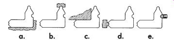
FIG. 7. Commercial radius gage and applications: (a) inspection of an inside radius tangent to two perpendicular planes; (b) inspection of a groove; (c) inspection of an outside radius tangent to two perpendicular planes; (d) inspection of a ridge segment; (e) inspection of roundness and diameter of a shaft.

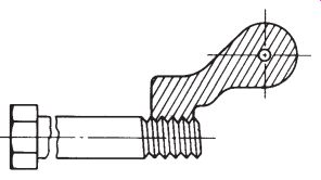
FIG. 8. Screw pitch gage and method of application.

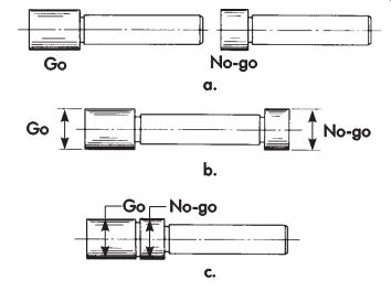
FIG. 9. AGD cylindrical plug gages used to inspect the diameter of holes.

Standard AGD plug gages generally have three methods of mounting gage members on the handle.

Smaller sizes are usually wire-type gages. The gage member is simply a straight blank or nib with no shoulder, taper, or threads. It is held in the handle by a setscrew or a collet chuck built into the handle, as shown in FIG. 10a. The advantage of this type of mounting is that the gage members are reversible when one end becomes worn, thus increasing the life of the gage.

FIG. 10b shows another type of mounting called the taper-lock design. The gage member is manufactured with a taper ground on one end.

The taper fits into a tapered hole in the handle much the same as a taper-shank drill fits into a drill-press spindle. This type is not reversible.

The third type of mounting is called the trilock design. This design is usually for larger gages. The gage member has a hole drilled through the center and is counterbored on both ends to receive a standard socket-head screw. Three slots are milled radially in each end of the gage member. The gage is held to the handle by means of a socket-head screw with the three slots engaging three lugs on the end of the handle as shown in FIG. 10c.

This type of gage is reversible.

Sometimes it is necessary to design special plug gages. There are many types, depending on the job requirement. A square, hexagonal, or octagonal hole requires a special plug gage.

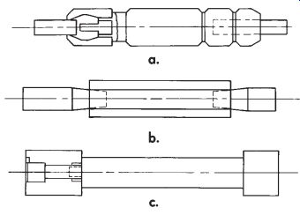
FIG. 10. AGD cylindrical plug gages: (a) reversible wire type, (b) taper-lock design (c) trilock design.

Internal splines require spline plugs designed in accordance with the standard from the American National Standards Institute, ANSI B92.1.

Internal threads require thread plugs designed in accordance with ANSI B1.2-1983 (R2007), etc.

FIG. 11 shows several special plug gages.

Ring Gage

Ring gages are usually used in pairs, consisting of go and no-go members, as shown in FIG. 12. They are fixed gages, and their design is covered by AGD standards.

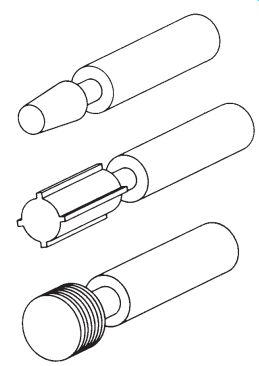
FIG. 11. Special plug gages used to inspect the profile or taper of holes. They check the individual feature elements but they do not check the boundary of perfect form.

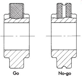
FIG. 12. Ring gage set used to inspect the diameter of shafts.

In sizes up to 1.51 in. (38.4 mm), the design is a plain ring, knurled on the outside diameter (OD) and lapped in the inside diameter (ID) to a close tolerance. The no-go member is identified by a groove around the OD of the gage. Some of these gages have a simple, thinner flange to reduce weight and increase rigidity.

Special ring gages are occasionally required. One example would be for the inspection of a shaft having a keyway, where a key-shaped segment added to a ring gage would allow gaging of shaft size, key-slot width, and depth at the same time. External splines require spline rings designed in accordance with the American Society of Mechanical Engineers standard, ASME B94.6-1984 (R2009). External threads require thread rings designed in accordance with ASME B1.2-1983 (R2007), etc. FIG. 13 shows several special ring gages.

Snap Gage

A snap gage is a fixed gage arranged with in side measuring surfaces for calipering diameters, lengths, thicknesses, or widths. Snap gages are available in a variety of types.

A plain adjustable snap gage is a complete external-caliper gage used for size control of plain external dimensions. It has an open frame with gaging members provided in both jaws. One or more pairs of gaging members can be set and locked to any predetermined size within the range of adjustment. The design of most types is covered by AGD standards. They are shown in FIG. 14.

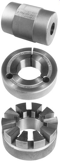
FIG. 13. Special ring gages to check profile or taper on parts.

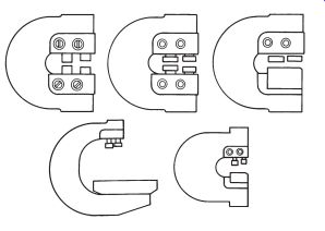
FIG. 14. AGD adjustable snap gages.

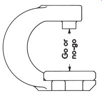
FIG. 15. Plain solid snap gage.

A plain solid snap gage, shown in FIG. 15, is another complete external-caliper gage used for controlling the size of plain external dimensions.

It has an open frame and jaws, with the latter carrying gaging members in the form of fixed, parallel, nonadjustable anvils.

The thread-roll snap gage, shown in Figure 9-16, is a complete external-caliper gage employed to control the size of the thread pitch diameter, lead of a thread, and thread form. It has an open frame and jaws in which gaging members are provided. One or more pairs of gaging members can be set and locked to a predetermined size within range of the thread to be checked.

Gaging members vary with different diameters and pitch or thread.

A form-and-groove or blade-type snap gage, as shown in FIG. 17, is a complete external-caliper gage used for controlling the size of grooves or checking close shoulder diameters. It has an open frame and adjustable blade anvils.

Many companies have master drawings of snap gages. The designer need only fill in the dimension needed to gage a part. These master drawings are then sent to gage manufacturers to fill the order. There are special cases when a single-purpose fixed snap gage is desired. For example, the OD of a narrow groove (as shown in FIG. 18) is checked with a special double-end snap gage designed to inspect the diameter.

At times, a snap gage may be better than a ring gage as an inspection tool. FIG. 19 illustrates how a ring gage may accept out-of-round work pieces that would be rejected by a snap gage.

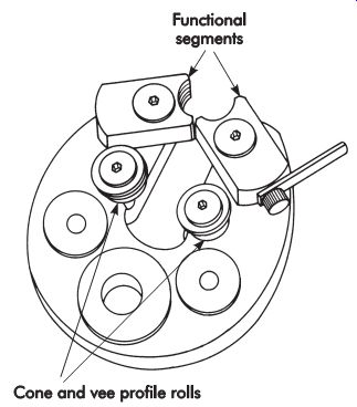
FIG. 16. Thread-roll snap gage.

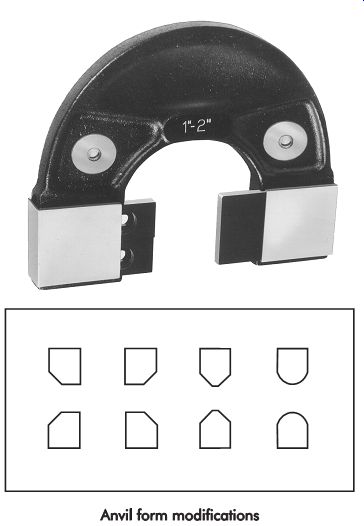
FIG. 17. Adjustable form-and-groove snap gage shown with typical anvil form modifications.

FIG. 18. Special snap gage.

Flush-pin Gage

The flush-pin gage is a simple mechanical device used to measure linear dimensions. The important parts of the gage are the body and a sliding pin or plunger. The indicating device is a step, ground either on the plunger or on the flush-pin body, equal to the total tolerance of the dimension.

When the gage is mounted on the workpiece, the position of the plunger can be checked visually or by fingernail touch.

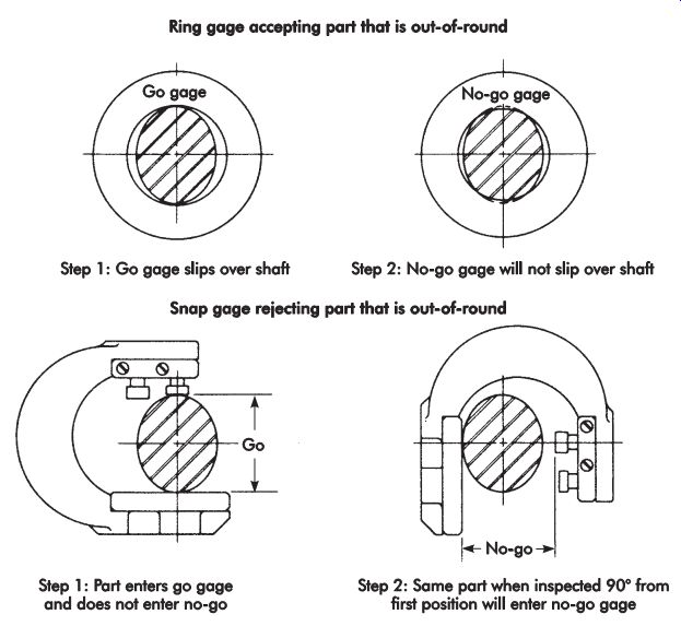
FIG. 19. Gage comparison.

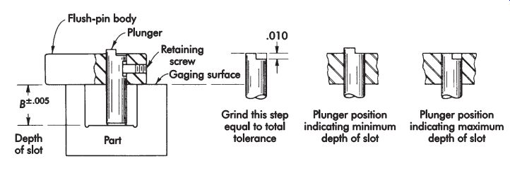
FIG. 20. Basic application of flush-pin gage indicating various positions of plunger.

FIG. 20 shows a slotted workpiece being checked with a flush-pin gage. Also shown are the relative positions of the plunger at the high and low limits of the depth. The flush-pin principle applied in this way is simple in operation, rugged and foolproof, does not require a master for presetting, and is economical when compared to micrometer or dial gaging methods. The dimension also could be checked with a depth micrometer. However, the depth micrometer requires a greater degree of operator skill, and there is the possibility of misreading the instrument.

FIG. 21 shows an inspection fixture containing two flush-pin gages and the work piece being checked. The first dimension being checked (X) is the distance from the center of the spherical radius to a flat surface. Dimension Y is between the center of the same spherical radius and over the outside of a roll (wire). A standard tooling ball in the base of the fixture locates the radius of the workpiece and provides the origin for both dimensions.

Amplification and Magnification of Error

As changes in dimension become too small to be easily measured, it is necessary to amplify or magnify them prior to measurement. This can be done mechanically, pneumatically, optically, or electronically.

As tolerances become tighter, primary gaging methods are not precise enough to detect the degree of error. An inspector may, for example, find that qualification of a workpiece no longer depends on whether a gage enters a hole, but on how much pressure is needed to insert the gage or whether the gage enters with too little pressure.

Inspection becomes more dependent on human judgment and is therefore less reliable.

A surface cannot be perfectly flat. Two parts cannot be exactly alike. Measured distances or quantities cannot be exactly equal. The inability of an inspection device to detect error proves only that the capability of the inspection device is limited. Error or deviation is always present.

The designer specifies what degree of error can be allowed. The inspector confirms that the error in the workpiece is within tolerance. Accuracy of measurement is limited by the accuracy of the standard used for comparison and the skill of the person making the comparison.

Indicating Gages and comparators

Indicating gages and comparators magnify the amount a dimension deviates above or below a standard to which the gage is set. Most indicate in terms of actual units of measurement, but some show only whether a tolerance is within a given range. The ability to measure to .000001 in. (25 nanometers [nm]) depends upon magnification, resolution, accuracy of the setting gages, and staging of the workpiece and instrument. Graduations on a scale should be .06-.10 in. (1.5-2.5 mm) apart to be clear. This requires magnification of 60,000-100,000 times for a .000001 in. (25 nm) increment; less is needed, of course, for larger increments.

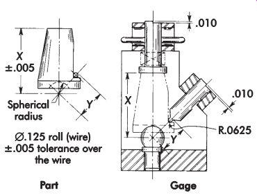
FIG. 21. Workpiece with flush-pin-type inspection fixture.

Mechanical, electronic, air, and optical sensors and circuits are available for any magnification needed and will be described in the following sections. However, measurements have meaning and are repeatable only if based upon reliable standards, like gage blocks, and if the support of the workpiece and instrument is stable. An example is that of equipment to trace the roundness of cylindrical parts. Either the probe or part must be rotated on a spindle that must run true with an error much less than the increment to be measured.

Dial Indicator

The dial indicator (FIG. 22) is perhaps the most widely used instrument for precise measurement. Basically, it consists of a probe, rack, pinion, pointer, dial, and case. The probe, which is attached to the end of the rack, is placed on the workpiece. A change in workpiece size changes

the position of the probe, which in turn moves the rack. The rack movement turns the pinion, which through a gear train causes the dial pointer to move. The graduated dial is calibrated for direct reading of variation from the nominal dimension.

Several amplification factors are involved.

Dial indicators are used for many kinds of measuring and gaging operations. They also serve to check machines and tools, alignments, and cutter runout. Dial indicators often are incorporated in special gages and measuring instruments.

Commercially available from many sources, standard models of dial indicators vary greatly in size, amplification ratio, mounting facilities, and precision. Inexpensive models are avail able for production use as well as very precise models for use in the gage crib.

An indicator gage has one primary advantage over a fixed gage: it shows how much a workpiece is oversize or undersize. When using an indicator as part of a gaging device, a master block sized to the nominal dimension to be checked must be used to preset the indicator to zero. Then, in applying the gaging device, the variation from zero, the nominal dimension, is read from the dial scale.

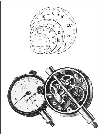
FIG. 22. Dial indicators.

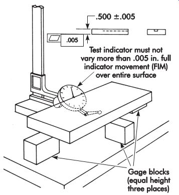
FIG. 23. Application of a dial indicator for inspecting flatness by placing the workpiece on gage blocks and checking full indicator movement (FIM).

FIG. 24. Squareness gaging fixture composed of standard inspection tools.

Extremely precise dial indicators are part of standard inspection equipment found in a gage crib, together with surface plates, parallels, V blocks, and vernier height gages. FIG. 23 shows a dial indicator being used to inspect the flatness of a workpiece mounted on gage blocks.

FIG. 24 shows standard inspection tools being used to check the squareness of a workpiece. In checking squareness or runout, the indicator is zeroed with the probe placed on the workpiece. If the same standard components are used directly as a height gage, the gage first must be zeroed to a known standard, such as a gage block or master.

If inspection is frequently needed, it may be expensive to tie up quality control equipment.

FIG. 25 shows a commercially available gaging fixture complete with surface, indicator, and stand. Attached centers and rolls for checking runout of centered or un-centered parts also are available.

Electric and Electronic Gages

Certain gages are called electric limit gages because they have the added feature of a rack stem that actuates precision switches. The switches connect lights or buzzers to show limits and may energize sorting and corrective devices.

An electronic gage gives a reading in proportion to the amount a stylus is displaced. It may also actuate switches electronically to control various functions. An example of an electronic gage and diagrams of the most common kinds of gage heads are shown in FIG. 26. The variable inductance or inductance-bridge transducer, a, has an alternating current (AC) fed into two coils connected into a bridge circuit. The reactance of each coil is changed as the position of the magnetic core changes. This changes the output of the bridge circuit. The vari able transformer or linear variable displacement transformer (LVDT) transducer, b, has two op posed coils into which currents are induced from a primary coil. The net output depends on the displacement of the magnetic core. The deflection of a strain-gage transducer, c, is sensed by the changes in length and resistance of strain gages on its surface. This is also a means for measuring forces. Displacement of a variable capacitance head, d, changes the air gap between the plates of a condenser connected in a bridge circuit. In every case, alternating current (AC) is fed into the gage as depicted in e. The output of the gage head circuit is amplified electronically and displayed on a dial or digital readout. The information from the gage may be recorded on tape or stored in a computer, a big advantage with this type of gaging.

Depending on capacity, range, resolution, quality, accessories, etc., electronic gages are priced from a little under $1,000 to many thousands of dollars.

An electronic height gage like the one shown in e with an amplifier and digital display is at the low end of the price scale. A digital-reading height gage like the instrument shown in f can be used for transferring height settings in increments of .00010 in. (0.0025 mm) with an accuracy of .000050 in. (0.00127 mm).

Electronic gages have several advantages: they are very sensitive (commonly reading to a few micrometers); output can be amplified as much as desired; a high-quality gage is quite stable; they generally can read either English or metric scales; a computer chip may be added to perform routine measurement algorithms; and they can be used as an absolute measuring device for thin pieces up through the range of the instrument. The amount of amplification can be switched easily, and three or four ranges are common for one instrument.

Two or more heads may be connected to one amplifier to obtain sums or differences of dimensions, as for checking thickness, parallelism, etc.

FIG. 27 shows electronic gage application data for a wide variety of measurements.

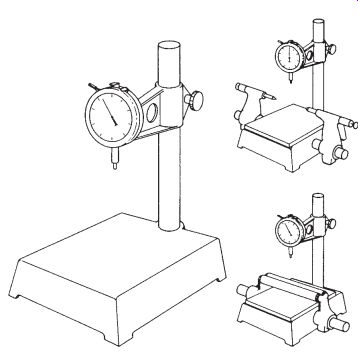
FIG. 25. Gaging fixture with accessories.

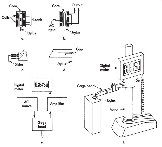
FIG. 26. Elements of electronic gages. Types of gage heads: (a) variable inductance; (b) variable transformer; (c) strain gage; (d) variable capacitance; (e) block diagram of typical electronic gage circuit; (f) one model of electronic gage.

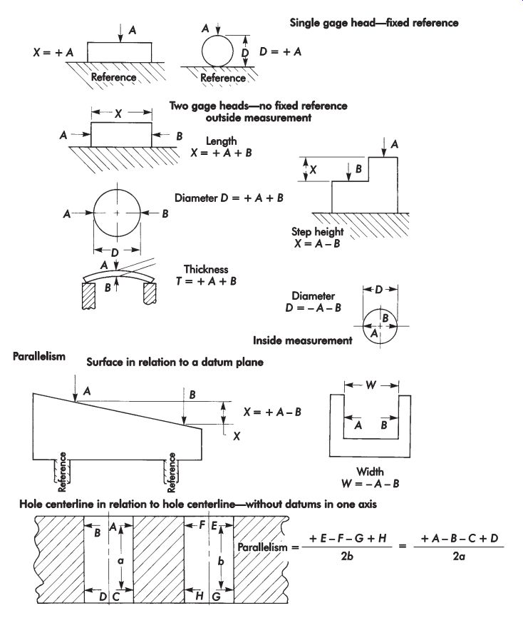
FIG. 27. Application data for electronic gaging.

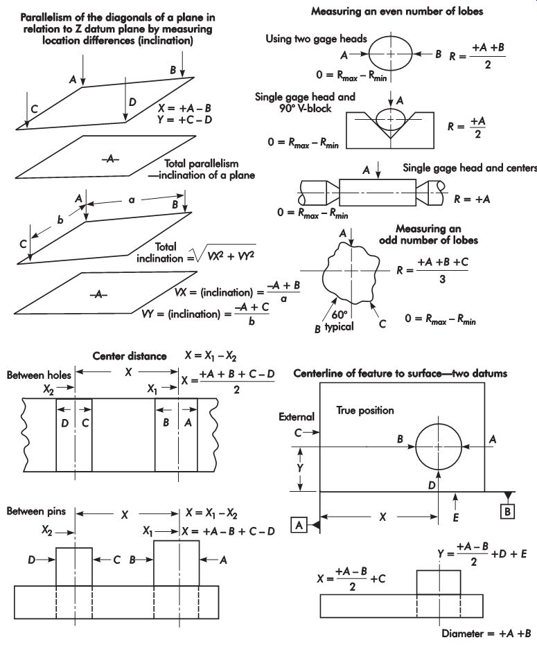
FIG. 27. (continued).

Air Gages

An air gage measures, compares, or checks dimensions by sensing the flow of air through the space between a gage head and workpiece surface. The gage head is applied to each work piece in the same way, and the clearance between the two varies with the size of the piece. The amount the airflow is restricted depends upon the clearance. Practically all inside and outside linear and geometric dimensions can be checked by air gaging.

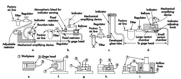
FIG. 28. Diagrams of air-gage principles. Air gage sensors: (a) back pressure; (b) differential; (c) flow; (d) venturi. Gage heads: (e) plug; (f) thickness; (g) taper; (h) cartridge or contact; (i) matching.

There are four basic types of air gage sensors shown in FIG. 28. All have a controlled constant-pressure air supply. The back-pressure gage, a, responds to the increase in pressure when the airflow is reduced. It can magnify from 1,000:1 to over 5,000:1, depending on range, but is somewhat slow because of the reaction of air to changing pressure. The differential gage, b, is more sensitive. Air passes through this gage in one line to the gage head and in a parallel line to the atmosphere through a setting valve. The pressure between the two lines is measured.

There is no time lag with the flow gage, c, where the rate of airflow raises an indicator in a tapered tube. The dimension is read from the position of the indicating float. This gage is simple, does not have a mechanism to wear, is free from hysteresis, and can amplify to over 500,000:1 without accessories. A venturi gage, d, measures the drop in pressure of the air flowing through a venturi tube. It combines the elements of the back-pressure and flow gages and is fast, but sacrifices simplicity. The basic gage sensor can be used for a large variety of jobs, but a different gage head and setting master are needed for almost every job and size.

A few of the many kinds of gage heads and applications are also shown in FIG. 28. An air gage is basically a comparator and must be set to a master for dimension or to two masters for limits. The common single gage head is the plug, which is being used to check the internal feature's diameter, as shown in e. In f the gage is checking the feature's outside diameter. In g, a taper is being checked on an internal feature. A multi-dimension gage has a set of cartridge or contact gage heads (FIG. 28h) to check several dimensions on a part at the same time. Air match gaging, depicted in FIG. 28i, measures the clearance between two mating parts. This provides a means of controlling an operation to machine one part to a specified fit with the other.

A major advantage of an air gage is that the gage head does not have to tightly fit the part.

A clearance of up to .003 in. (0.08 mm) between the gage head and workpiece is permissible, even more in some cases. Thus no pressure is needed between the two to cause wear, and the gage head may have a large allowance for any wear that does occur. The flowing air helps keep surfaces clean.

The lack of contact makes air gaging particularly suitable for checking against highly finished and soft surfaces. Because of its loose fit, an air gage is easy and quick to use. An inexperienced worker can measure the diameter of a hole to .000001 in. (25 nm) in a few seconds with an air gage; the same measurement to .001 in. (25 um) with a vernier caliper by a skilled inspector may take up to 1 minute. The faster types of air gages are adequate for high-rate automatic gaging in production.

Air gaging is subject to varying shop air pressures, humidity, temperature, etc., which must be taken into account when designing these systems.

Optical Projection Gaging

Optical projection is a method of measurement and gaging using a precision instrument known as an optical projector or comparator. Optical gaging is gaging by sight rather than feel or pres sure. The measurement or gaging is performed by placing a workpiece in the path of a beam of light and in front of a magnifying-lens system, thereby projecting an enlarged silhouette shadow of the object upon a translucent screen as illustrated in FIG. 29.

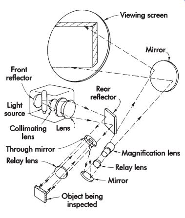
FIG. 29. Optical projection gaging principle.

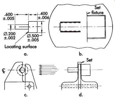
FIG. 30. Optical gage setup: (a) workpiece; (b) chart gage; (c) side view of holding fixture; (d) front view of holding fixture.

Measurement of a workpiece normally requires a chart gage with Reference lines in two planes. In gaging applications, a precisely scaled layout of the contour of the part to be gaged, usually with tolerance limits, is drawn on the screen. FIG. 30 shows a workpiece with the chart gage used for its inspection.

Optical gages are almost unaffected by wear.

There is no wear to a light beam, and any fixture wear can be compensated for by repositioning to the setting point. Little operator skill is required; no touching skill or sensitivity is needed.

Dimensions can be changed on the screen easily and quickly. The chart provides exact duplication. Several dimensions can be checked at the same time, eliminating too much handling of the part.

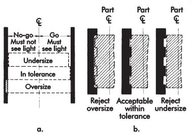
FIG. 31. Chart gage segments: (a) maximum and minimum tolerance lines; (b) close-tolerance bridge arrangement.

Most optical projectors have standard magnification of 10× up to 100×. The effective area that can be projected through a given lens system can be determined by dividing the screen diameter by the magnification of the lens being used. For example, a comparator with a 14-in. (356-mm) diameter screen, using 10× magnification, will project the complete area of a 1.400-in. (35.56 mm) diameter specimen at one setting.

A chart gage is an accurately scribed, magnified, outline drawing of the workpiece to be gaged.

It contains all the contours, dimensions, and tolerance limits necessary. The chart is made of glass or plastic. For short and quick checks, drafting paper can be used. However, paper should not be used consistently because it shrinks with changes of weather. Chart layout lines should be dark black, sharply defined, and from .006-.020 in. (0.15-0.51 mm) wide for best legibility. Dimensions normally extend to the center of the lines.

When maximum and minimum tolerance lines are used, the magnification should be high enough to maintain a minimum of .020 in. (0.51 mm) spacing between the lines. For closer tolerance checking, special lines or bridge arrangements, based on gaging to the edge of the lines, are often used. FIG. 31 shows two portions of a chart gage. The first portion, a, uses maximum and minimum tolerance lines. The second portion, b, has a close-tolerance bridge arrangement.

Workholding equipment includes vises for flat workpieces and staging centers for round workpieces, such as shafts and cylindrical parts with machined centers. V-blocks, in a range of sizes, are mounted on bases to clamp to projector worktable slots. Diameter capacities run from 0-5 in. (0-127 mm).

Automatic Gaging Systems

As industrial processes are automated, gaging must keep pace. Automated gaging is per formed in two general ways. One is in-process or on-the-machine control by continuous gaging of the work. The second way is post-process or after-the-machine gaging control. Here, the parts coming off the machine are passed through an automatic gage. A control unit responds to the gage to sort pieces by size and adjust or stop the machine if parts are found out of limits.

Coordinate Measuring Machines

The coordinate measuring machine (CMM) is a flexible measuring device capable of providing highly accurate dimensional position information along three mutually perpendicular axes.

This instrument is widely used in manufacturing industries for post-process inspection of a large variety of products and their components.

It is also effectively used to check dimensions on a variety of process tooling, including mold cavities, die assemblies, assembly fixtures, and other workholding or tool positioning devices. A system diagram of a measurement processor for automatic direct computer control (DCC) of a CMM is shown in FIG. 32.

Moving Bridge CMM

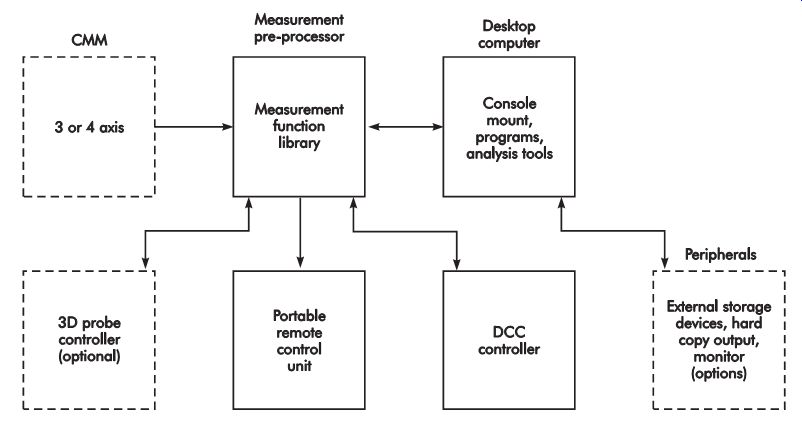
FIG. 32. Measurement processor for a direct, computer-controlled, coordinate measuring machine.

The two most common structural configurations for CMMs are the moving bridge and the cantilever. The basic elements and configuration of a typical moving-bridge type CMM are shown in FIG. 33. The base or worktable of most CMMs is constructed of granite or some other ceramic material to provide a stable work-locating surface and an integral guideway foundation for the superstructure. As indicated in FIG. 33, the two vertical columns slide along precision guideways on the base to provide Y-axis movement. A traveling block on the bridge gives X-axis movement to the quill, and the quill travels vertically for a Z-axis coordinate. The moving elements along the axes are supported by air bearings to minimize sliding friction and compensate for any surface imperfections on the guideways.

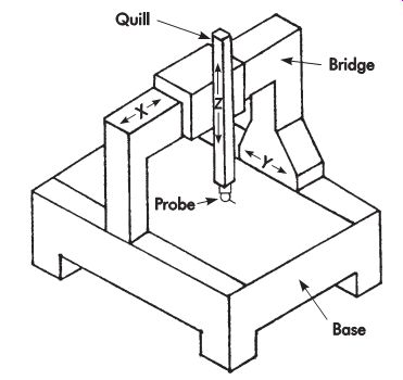
FIG. 33. Typical moving-bridge coordinate measuring machine configuration.

Movement along the axes can be accomplished manually on some machines by light hand pres sure or rotation of a handwheel. Movement on more expensive machines is accomplished by axis drive motors, sometimes with joystick control.

Direct computer controlled CMMs are equipped with axis drive motors, which are program controlled to automatically move the sensor element (probe) through a sequence of positions.

To establish a Reference point for coordinate measurement, the CMM and probe being used must be datumed. In the datuming process, the probe, or set of probes, is brought into contact with a calibrated sphere located on the worktable.

The center of the sphere is then established as the origin of the X-Y-Z axes coordinate system.

The coordinate measuring machine shown in FIG. 34 has a measuring envelope of about 18 × 20 × 16 in. (0.5 × 0.5 × 0.4 m) and is equipped with a disengagable drive that enables the operator to toggle between manual and DCC. It has a granite worktable and the X-beam and Y-beam are made of an extruded aluminum to provide the rigidity and stability needed for ac curate measuring. The measurement system has a readout precision of .00004 in. (1 um) and the DCC system can be programmed to accomplish 45-60 measurement points/min. A CMM of this size can be equipped with computer support, joystick control, electronic touch probe, or video camera for noncontact measurement.

Contacting Probes

CMM measurements are taken by moving the small stylus (probe) attached to the end of the quill until it makes contact with the surface to be measured. The position of the probe is then observed on the axes readouts. On early CMMs, a rigid (hard) probe was used as the contacting element. The hard probe can lead to a variety of measurement errors, depending on the contact pressure applied, deflection of the stylus shank, etc. These errors are minimized by the use of a pressure-sensitive device called a touch-trigger probe.

The touch-trigger probe permits hundreds of measurements to be made with repeatabilities in the .00001-.00004 in. (0.25-1.0 ?m) range. Basically, this type of probe operates as an extremely sensitive electrical switch that detects surface contact in three dimensions. The manual index able touch-trigger probe shown in FIG. 35 can be used to point and probe without redatuming for each position measured. A probe of this type can be used on manually operated CMMs.

Motorized probe heads are available for use on DCC CMMs.

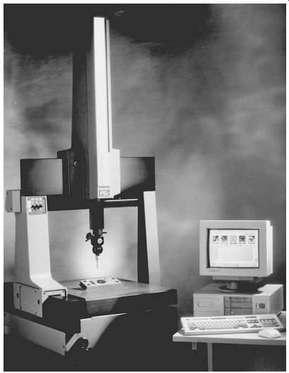
FIG. 34. Coordinate measuring machine.

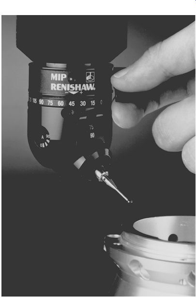
FIG. 35. Manual indexable probe.

Noncontacting sensors

Many industrial products and components that are not easily and suitably measured with surface-contacting devices may require the use of noncontact sensors or probes on CMMs to obtain the necessary inspection information.

This may include two-dimensional parts such as circuit boards and very thin stamped parts; extremely small or miniaturized microelectronic devices and medical instrument parts; and very delicate, thin-walled products made of plastic or other lightweight materials.

There are several noncontacting sensor systems available that have been adapted either individually or in combination with the coordinate measuring process. All of these involve optical measuring techniques and include microscopes, lasers, and video cameras. The automated, three-dimensional, video-based, coordinate measuring system appears to offer many advantages because of its ability to accomplish multiple measurement points within a single video frame. Thus, it is often possible to obtain data from several hundred coordinate points with a video measuring system in the same time it would take to obtain a single-point measurement with a conventional touch-probe system. A large number of points on a part can be imaged with charged couple device (CCD) video cameras, depending on the optical view and array or pixel size of the camera. For example, one commercially available system has a field of view range from .02-.30 in. (0.5-7.6 mm) with a 756 × 581 pixel array and can image the field of view at 30 video frames/second.

Video-based systems do not have the same throughput advantage for height (Z axis) measurements as they do for two-dimensional (X-Y) measurements because of the time involved for focusing. On some machines, this disadvantage is overcome by integrating laser technology with the video system.

The multi-sensor coordinate measuring ma chine (MSCMM) shown in FIG. 36 incorporates three sensing technologies-optical, laser, and touch probe-for highly accurate noncontact and/or contact inspection tasks. The machine uses two quills or measuring heads to accomplish high-speed data acquisition within a four-axis (X, Y, Z1, Z2) configuration, thus permit ting noncontact or contact inspection of virtually any part in a single setup.

The sensing head on the left quill in FIG. 36 contains an optical/laser sensor with a high resolution CCD video and a coaxial laser. The video camera has advanced image-processing capabilities via its own microprocessor, enabling sub-pixel resolutions of 2 ?in. (0.05 ?m). The coaxial laser shares the same optical path as the video image and assists in focusing the CCD cam era. This eliminates focusing errors associated with optical systems and increases the accuracy of Z measurements. Single-point measurements can be obtained in less than 0.2 seconds, and high-speed laser scanning/digitizing can be accomplished at up to 5,000 points/second.

The right-hand quill of FIG. 36 contains the Z2-axis touch-probe sensor used to inspect features that are either out of sight of the optical/laser sensor or better-suited to be measured via the contact method.

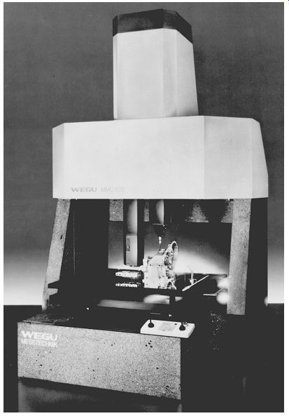
FIG. 36. A multi-sensor coordinate measuring ma chine with optical, laser, and touch probes for noncontact and contact measurements.

The machine in FIG. 36 is being used to inspect a valve body with the Z1-axis optical/ laser probe and a transmission case with the Z2-axis touch probe. It is a bench-top type with a maximum measuring range of about 35 in. (900 mm), about 32 in. (800 mm), and about 24 in. (600 mm) for the X, Y, and Z1 and Z2 axes, respectively. Positioning of the moving elements is accomplished by backlash-free, recirculating ball lead screws and computer-controlled direct current (DC) motors. Position information is provided by high-precision glass scales.

Measuring with Light Rays

Light waves of any one kind are of invariable length and are the standards for ultimate measures of distance. Basically, all interferometers divide a light beam and send it along two or more paths. Then the beams are recombined and al ways show interference in some proportion to the differences between the lengths of the paths.

One of the simplest illustrations of the phenomenon is the optical flat and a monochromatic light source of known wavelength. The optical flat is a plane lens, usually a clear, fused quartz disk from about 2-10 in. (51-254 mm) in diameter and .5-1.0 in. (13-25 mm) thick. The faces of a flat are accurately polished to nearly true planes; some have surfaces within .000001 in. (25 nm) of true flatness.

Helium is commonly used in industry as a source of monochromatic or single-wavelength light because of its convenience. Although helium radiates a number of wavelengths of light, the portion emitted with a wavelength of .00002313 in. (587 nm) is so much stronger than the rest that other wavelengths are practically unnoticeable.

The principle of light-wave interference and the operation of the optical flat are illustrated in FIG. 37a, wherein an optical flat is shown resting at a slight angle on a workpiece surface.

Energy in the form of light waves is transmitted from a monochromatic light source to the optical flat. When a ray of light reaches the bottom surface of the flat, it is divided into two rays. One ray is reflected from the bottom of the flat toward the eye of the observer, while the other continues downward, is reflected, and loses one-half wavelength on striking the top of the workpiece.

If the rays are in-phase when they re-form, their energies reinforce each other, and they appear bright. If they are out-of-phase, their energies cancel and they are dark. This phenomenon produces a series of light and dark fringes or bands along the workpiece surface and the bottom of the flat, as illustrated in FIG. 37b. The distance between the workpiece and the bottom surface of the optical flat at any point determines which effect takes place.

If the distance is equivalent to some whole number of half wavelengths of the monochromatic light, the reflected rays will be out of-phase, thus producing dark bands. This condition exists at positions X and Z of FIG. 37a. If the distance is equivalent to some odd number of quarter wavelengths of the light, the reflected rays will be in-phase with each other and produce light bands. The light bands would be centered between the dark bands. Thus a light band would appear at position Y in FIG. 37a.

Since each dark band indicates a change of one-half wavelength in distance separating the work surface and flat, measurements are made simply by counting the number of these bands and multiplying that number by one-half the wavelength of the light source. This procedure may be illustrated by the use of FIG. 37b.

There, the diameter of a steel ball is compared with a gage block of known height. Assume a monochromatic light source with a wavelength of 23.13 ?in. (0.6 ?m). From the four interference bands on the surface of the gage block, it is obvious that the difference in elevations of positions A and B on the flat is equal to (4 × 23.13)/2 or 46.26 ?in. ([4 × 0.6]/2 or 1.2 ?m). By simple proportion, the difference in elevations between points A and C is equal to (46.26 × 2.5)/0.5 = 231.3 ?in. ([1.2 × 64]/13 = 5.9 ?m). Thus, the diameter of the ball is 0.750 × .0002313 = .0001734 in. (19.05 × 0.005875 = 0.111919 mm).

Optical flats are often used to test the flatness of surfaces. The presence of interference bands between the flat and the surface being tested is an indication that the surface is not parallel with the surface of the flat. The way dimensions are measured by interferometry can be explained by moving the optical flat of FIG. 37a in a direction perpendicular to the workpiece face or mirror.

It is assumed that the mirror is rigidly attached to a base, and the optical flat is firmly held on a true slide. As the optical flat moves, the distance be tween the flat and mirror changes along the line of traverse, and the fringes appear to glide across the face of the flat or mirror. The amount of movement is measured by counting the number of fringes and fraction of a fringe that pass a mark.

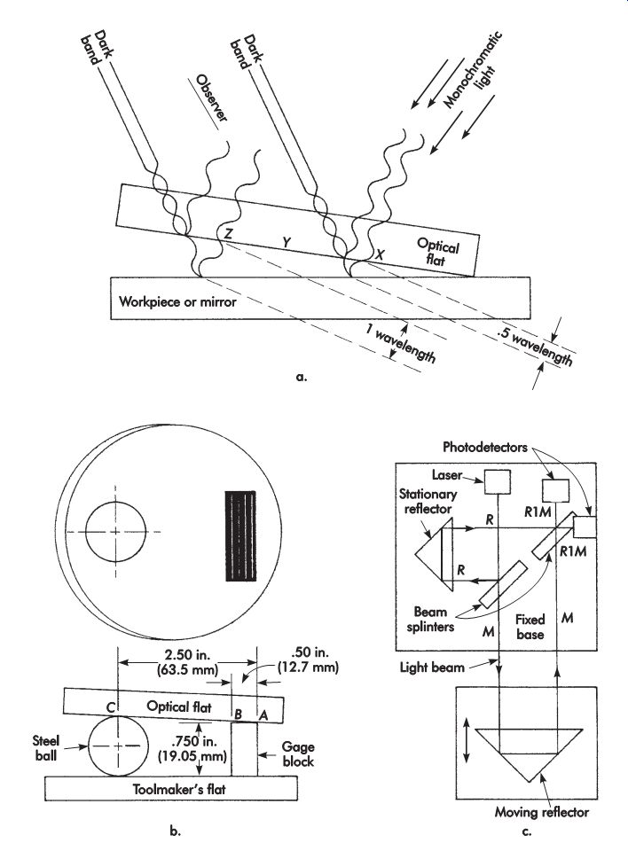
FIG. 37. (a) Light-wave interference with an optical flat; (b) application of an optical flat; (c) diagram of an interferometer.

It is difficult to precisely superimpose a real optical flat on a mirror or the end of a piece to establish the end points of a dimension to be measured. This difficulty is overcome in sophisticated instruments by placing the flat elsewhere and by optical means reflecting its image in the position relative to the mirror in FIG. 37a. This creates interference bands that appear to lie on the face of and move with the workpiece or mirror.

The image of the optical flat can be merged into the planes of the workpiece surfaces to establish beginning and end points of dimensions.

A simple interferometer for measuring movements of a machine tool slide to millionths of an inch (nanometers) is depicted in FIG. 37c. A strong light beam from a laser is split by a half mirror. One component becomes the Reference, R, and is reflected solely over the fixed machine base.

The other part, M, travels to a reflector on the machine slide and is directed back to merge with ray R at the second beam splitter. Their result is split and directed to two photodetectors. The rays pass in and out of phase as the slide moves. The undulations are converted to pulses by an electronic circuit; each pulse stands for a slide movement equal to one-half the wavelength of the laser light.

The signal at one photodetector leads the other according to the direction of movement.

When measurements are made to millionths of an inch (nanometers) by an interferometer, they are meaningful only if all causes of error are closely controlled. Among these are temperature, humidity, air pressure, oil films, impurities, and gravity. Consequently, a real interferometer is necessarily a highly refined and complex instrument; only its elements have been described here.

Optical Tooling

Telescopes and accessories to establish precisely straight, parallel, perpendicular, or angled lines are called optical tooling. Two of many applications are shown in FIG. 38a and b. One is to check the straightness and truth of the ways of a machine-tool bed at various places along the length. The other is to establish Reference planes for measurements on a major aircraft or missile component. Such methods are especially necessary for large structures. Accuracy of one part in 200,000 is regularly realized; this means that a point at a distance of 100 in. (2.5 m) can be located to within .0005 in. (13 ?m). Common optical-tooling procedures are auto-collimation, autoreflection, planizing, leveling, and plumbing.

Auto-collimation

Autocollimation is performed with a telescope having an internal light that projects a beam through the cross-hairs to a target mirror as indicated in FIG. 38a. If the mirror face is truly perpendicular to the line of sight, the cross-hair image will be reflected back on itself.

The amount the reflected image deviates from the actual reticle image is an indication of the tilt in the target. A target may have a cross-line pattern for alignment with the line of sight. An autocollimated image is not clear for distances over 50 ft (15.2 m), and then a somewhat less accurate method must be used.

Autoreflection

Autoreflection is performed with an optical flat containing a cross-line pattern mounted on the end of the illuminated telescope and focused to twice the distance of the target mirror. Then, if the mirror is perpendicular to the line of sight, the pattern of the flat is reflected in coincidence with the cross-hairs in the telescope.

Planizing

Planizing is composed of fixing planes at 90° with other planes or with a line of sight. This may be done from accurately placed rails on which transits are mounted in a tooling dock as indicated in FIG. 38b. A transit is a telescope mounted to swing in a plane perpendicular to a horizontal axis. Square lines also may be established with an optical square or planizing prism mounted on or in front of a telescope as depicted in FIG. 38c. Angles may be precisely set by autocollimating on the precisely located faces of an optical polygon as in FIG. 38d.

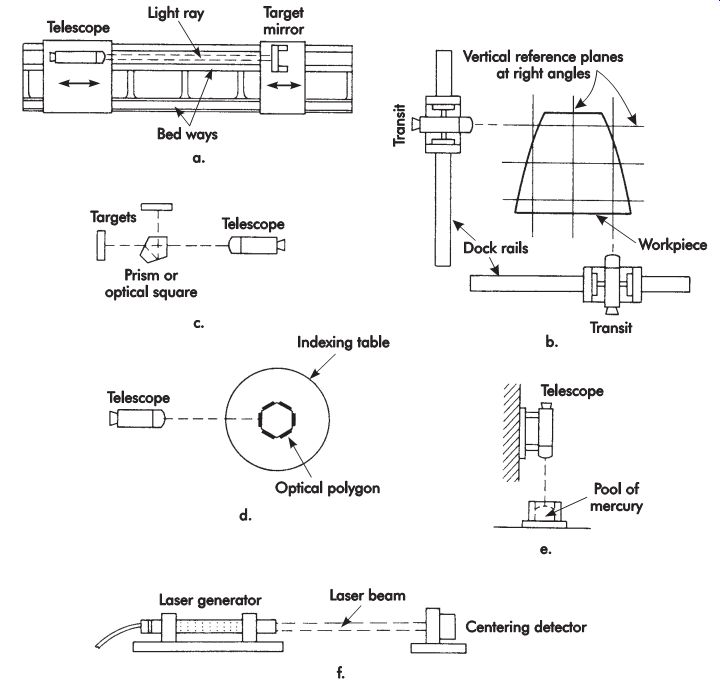
FIG. 38. Optical tooling: (a) autocollimation, or autoreflection, for checking the straightness of the ways on a machine-tool bed; (b) planizing to establish Reference planes in a tooling dock; (c) establishing a line at right angles to a line of sight by means of an optical square; (d) collimating the faces of an optical polygon to check angles on an index table; (e) example of a plumbing operation to establish a vertical line; (f) use of a centering detector to establish alignment with the center of a laser beam.

Leveling and Plumbing

Leveling establishes a horizontal line of sight or plane. This may be done with a telescope fitted with a precision spirit level to fix a horizontal line of sight. A transit or sight level so set may be swiveled around a vertical axis to generate a horizontal plane. Plumbing, shown in FIG. 38e, consists of autocollimating a telescope from the surface of a pool of mercury to establish a vertical axis.

Laser Light Beam

Advanced optical tooling uses the intense light beam of a laser. A centering detector, shown in FIG. 38f, has four photocells equally spaced (top and bottom and on each side) around a point. Their output is measured and becomes equalized when the device is centered with the beam. This provides a means to obtain alignment with a straight line. Squareness may be established by passing a laser beam through an optical square.

Gaging Methods

Many different part attributes can be measured or checked using a number of the gaging devices previously described. Following is a discussion of the most common devices and methods used in gaging and measurement.

Flatness

Various methods of checking flatness are avail able. Method selection depends on the accuracy required, size of the part, and time available to make the check. Flatness cannot be easily checked by functional methods.

One of the most widely used methods for checking flatness is direct contact. With this method, the part being checked is brought into direct contact with a Reference plane of known flatness that has been covered with a thin coating of layout fluid (Prussian blue). The high spots on the part are indicated by the transfer of the blue dye. This method, however, does not lend itself to geometrics because the results are not measurable.

Another common method for checking flatness is with an indicator, stand, leveling device, and a surface plate of known flatness, as shown in FIG. 39. With this method, the surface to be checked is first adjusted with the leveling device as shown by the indicator to establish the most accurate plane possible, parallel to the surface plate. The entire surface then is explored with the indicator to determine the full indicator movement (FIM), which is the measure of flatness.

Straightness

Straightness of surface elements can be checked by various methods, depending on the required accuracy and part size.

One common method of checking element straightness is with a straightedge or surface plate of known straightness and gage blocks or thickness stock. With this method, the part to be checked is supported at two places equidistant from the surface, and the differences from parallel are measured with gage blocks or an indicator set up to determine the FIM or equivalent. Cylindrical parts and narrow surfaces sometimes are placed directly on the surface plate and the differences checked with thickness stock. For small tolerances, element straightness can be checked by placing a toolmaker's knife edge directly on the part as shown in FIG. 40. Differences in element straightness are indicated by the presence and width of light gaps. Deciding element straightness by this method, however, generally does not provide measurable results.

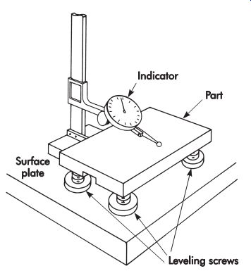
FIG. 39. Leveling a part.

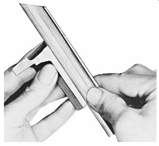
FIG. 40. Checking surface element straightness with a toolmaker's straightedge.

A more practical check can be made with a measuring machine as shown in FIG. 41.

The tracking accuracy of these machines permits checking, with a high degree of resolution, the locations of many separate points along the surface.

Numerical information is provided on any out-of straight condition. When these machines are computer-assisted, precision setups are not needed and the condition can be displayed directly.

Large, accurate straightness measurements are made with precision levels, electronic levels, autocollimators, or alignment telescopes using the same methods described for checking flatness.

When the straightness of an axis is specified as maximum material condition (MMC), it can be checked with a functional gage. A gage to check the straightness of a center plane MMC would basically consist of two parallel surfaces, .312 in. (7.92 mm) apart, through which the part must pass to be acceptable.

Circularity

Although the common method for checking circularity uses a V-block or checking from centers, these methods are not recommended. The many possible sources of error, such as lobing, angle of V-block, center misalignment, etc., contribute to inaccurate reading of the conditions.

Circularity should be checked with a precision rotating spindle, rotating table, or circular tracing instrument. Measurement is made by centering the part on the table, establishing an axis, and placing a stylus in contact with the surface of the circular cross-section. The stylus contacts the surface normal to the axis being examined to pick up, magnify, and display departures from roundness for determination of any out-of-round condition.

These instruments can be equipped with auto-centering capability, eliminating the need to precisely align the part before checking. Properly equipped, these instruments can be used for the complete analysis of circular sections.

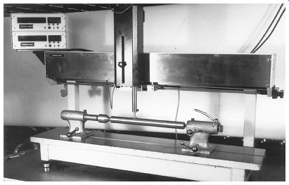
FIG. 41. Checking straightness while the part is held motionless.

Along with any of the previously mentioned checks, elements of the surface must be measured separately to ensure that they are within the specified size tolerance and boundary of perfect form at MMC.

Cylindricity

Cylindricity is checked with the same equipment used to check roundness, except that roundness readings must be taken at a number of sections along the entire length of the part.

Reading locations are placed in such a way as to establish a common axis from which a tolerance zone can be established and measurements made to determine whether they fall within the tolerance zone specified. As with the circularity checks, elements of the cylindrical surface must be measured separately to ensure that they are within the specified size tolerance and boundary of perfect form at MMC.

Profile of a line or surface

Many profiles are checked with contour gages having the opposite form of the nominal con tour of the part. Limit gages representing the go and no-go sizes of the part as determined by the maximum and minimum material condition, which compounds the effects of form and size tolerances, are also used. However, neither of these methods is suitable for geometrics.

One suitable method is to compare the part with a master part that conforms exactly to the basic dimensions of the part. A method to do this is shown in FIG. 42.

Cams and other profiles that can be rotated are measured directly with long-range digital reading sensors. Readings are compared with a perfect master in the memory of a microcomputer, and any out-of-tolerance conditions are printed along with their locations.

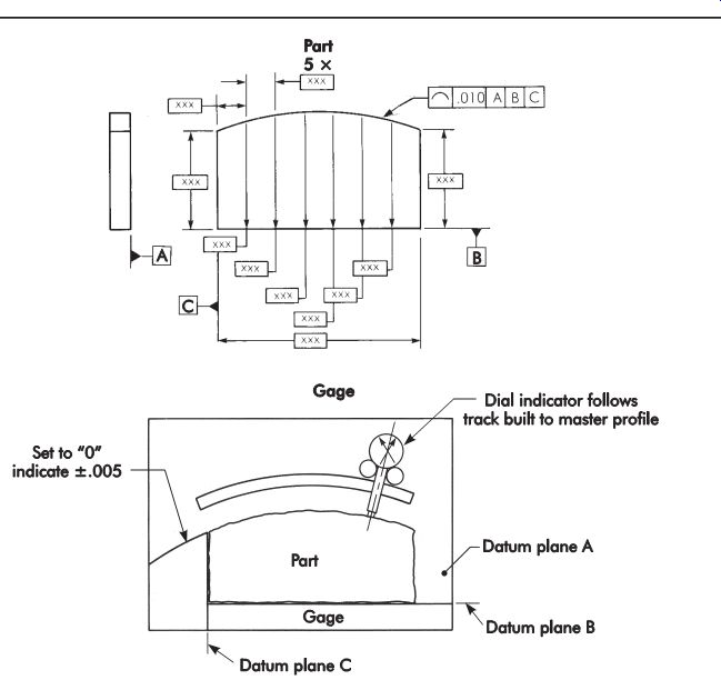
FIG. 42. Checking profile-indicator following a master profile.

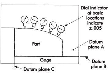
FIG. 43. Checking profile-fixed indicators set to master part.

FIG. 43 shows another generally accepted method that uses a fixture with several indicating devices mounted side by side in a plane containing the profile to be inspected. The indicators must be set with a master representing the basic profile. Conformance of the part is easily determined by reading the part differences directly from the indicators or display unit.

The best way to check small complex profiles is with an optical projector using one of the methods previously described. However, low spots cannot be detected. To check profile contours, an optical comparator with a contour projector tracer attachment, as shown in FIG. 44, may be used.

Perpendicularity (squareness)

The most common method of checking perpendicularity of surfaces is by direct comparison with gages of known squareness, such as the precision square. To make this check, the square and the part are placed in contact with each other while resting on a surface plate. Out-of-squareness is determined by measuring the gap between the square and sections along the part with a thickness gage, as shown in FIG. 45.

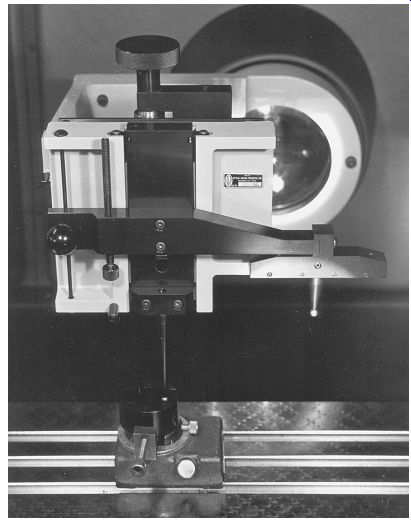
FIG. 44. Optical comparator with a contour projector tracer attachment.

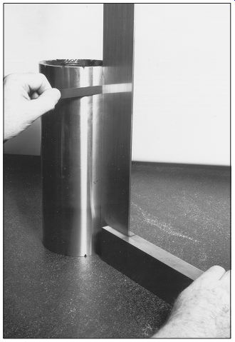
FIG. 45. Checking squareness with a square.

Another direct contact method uses a direct reading cylindrical square. It has one face-off angle and dotted curves and graduations etched on the surface indicating the amount of out-of squareness for the bounded area. In use, the part and the cylindrical square are placed on a surface plate and brought together while rotating the cylindrical square to produce the smallest light gap. The number of the topmost dotted curve in contact with the part surface indicates the squareness error.

Another widely used method for checking perpendicularity confirms whether two preselected points on the vertical surface of the part are in a common plane at right angles to the surface plate on which the part and gage are resting. Measurement is made by contacting the part with the spherical base of the comparator square and the probe of the indicator mounted in the stand, as shown in FIG. 46. Before the measurement is made, the indicator is set to zero with the aid of the cylindrical square shown. With this method, multiple checks must be made at varying heights to get an indication of the complete surface condition. The squareness gage, shown with its master in FIG. 47, measures in a similar way except that the part's surface can be completely indicated in a vertical manner due to the precision guideways built into the gage. Accuracy is maintained by comparing and adjusting the squareness to the master gage.

Large, accurate perpendicular measurements generally are made with an autocollimator, optical square, and reflector stand using a setup such as the one shown in FIG. 48. Sometimes special fixtures are used, such as those shown in FIG. 49, which permit the concerned feature to be searched with indicating depth gages. None of these methods, however, are applicable to the other examples shown.

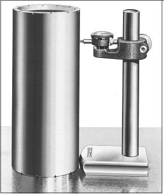
FIG. 46. Transfer inspection of squareness using cylindrical and comparator squares. (Taft Pierce)

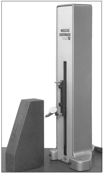
FIG. 47. Squareness gage and master.

Perpendicularity specifications, such as cylindrical size feature regardless of feature size (RFS) and non-cylindrical feature RFS, cannot be checked by functional gaging. They also would be difficult to check economically by other means. This is because a number of direct or differential measurements would have to be made, depending on the feature basic form errors, just to determine the attitude of the axis or median plane. For small quantities, a simple staging fixture could be used to quickly arrange the datum surface so the concerned feature is properly lined up with the surface plate. A height stand and indicator, as shown in FIG. 50, could be used to easily check squareness. For production quantities, fixtures generally are designed with air or electronic probes properly positioned and connected to determine the squareness of the axis or median plane to the datum surface.

Other perpendicularity specifications, such as cylindrical size feature and maximum material condition (MMC), could be checked with a functional gage, as shown in FIG. 51.

Angularity

Angularity tolerance cannot be checked with functional gaging. Angularity control can be called out at MMC or least material condition (LMC). RFS only applies to feature sizes.

Most short-run parts are checked for angularity with standard surface-plate methods. Sine plates or simple staging fixtures are used to place the datum surface of the concerned feature in proper alignment with the surface plate.

For production quantities, fixtures are generally designed with specifically located and interrelated air or electronic probes that check and display any out-of-tolerance condition of the feature angle being checked.

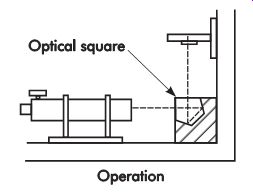
FIG. 48. Checking perpendicularity with an auto collimator.

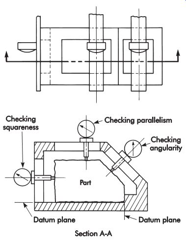
FIG. 49. Checking squareness, parallelism, and angularity with indicating depth gages.

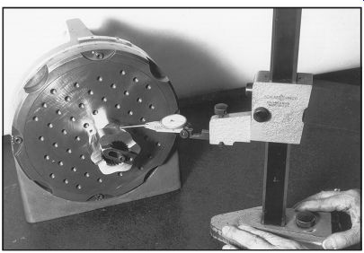
FIG. 50. Checking perpendicularity with a height stand and an indicator.

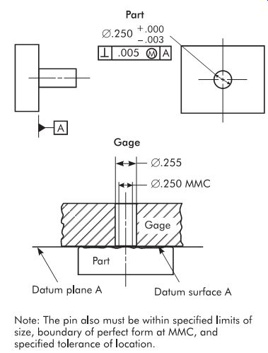
FIG. 51. Functional gage to check perpendicularity, cylindrical size feature, and MMC.

Large, accurate angularity measurements generally are made with an autocollimator or special fixtures and indicating depth gages in a manner similar to those shown for checking perpendicularity in FIGs. 48 and 49.

Parallelism

Parallelism of a surface generally is checked by placing the datum of the part on a surface plate and searching for any out-of-parallel conditions with a height stand and indicator.

Many times, a part, because of its geometry, must be placed in a special fixture to check perpendicularity, angularity, location, etc. In these cases, a check for parallelism generally is incorporated in the same fixture shown in FIG. 49.

When parallelism concerns cylindrical size features or datums, the inspection becomes more difficult, especially when the feature, datum, or both, are RFS. Here again, standard layout methods using a surface plate, height stand, and indicator can be used for small quantities as long as the inspector understands the meaning expressed by the feature control symbol. FIG. 52 shows an inspection gage design used to check the parallel ism of cylindrical size features.

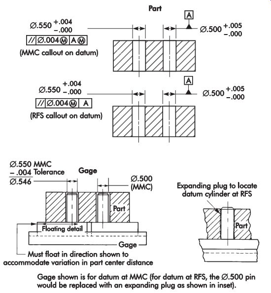
FIG. 52. Gage for checking parallelism-cylindrical size feature.

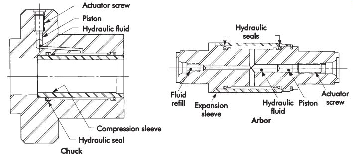
FIG. 53. Hydraulically actuated arbors and chucks.

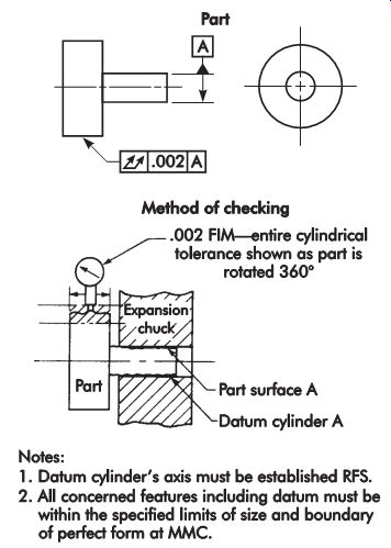
FIG. 54. Checking runout from an OD datum.

Runout

Checking runout on a part on which the datum axis is established by two part centers is relatively simple and easily understood. Low-production parts are generally mounted between the centers of a bench center and rotated 360° with a dial indicator (FIG. 22) in contact with the surface to be checked. For high production, special fixtures with several air, electronic, or mechanical indicators are generally more practical.

Parts where the datum axis is established by two functional diameters are generally checked in the same manner, except that the datum is established by closing in on the datum features with expanding chuck-like devices, as shown in FIG. 53. The reading is then taken in the same manner as from centers. Another method widely used with electronic gaging allows the part to be mounted in any suitable fashion, while indicating the datums as well as the features to be checked. The readings then are adjusted electronically within the equipment and the runout can be displayed directly.

Methods for checking the runout on parts where the datum is established from a diameter, or a combination of datum diameter and functional face, are shown in FIGs. 54, 55, and 56. The cylindrical datums must be established by chuck-like devices or electronically as noted previously since runout always is RFS.

When checking runout, all features of the part also must be measured separately to ensure they are within the specified size limits and the boundary of perfect form at MMC.

Position

Functional gaging can be used when position tolerance is applied on an MMC basis.

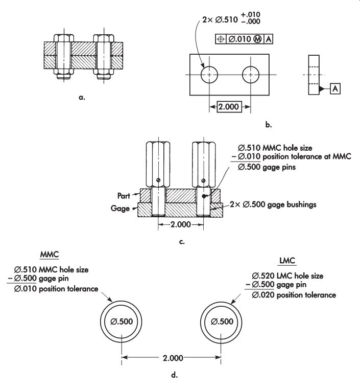
FIG. 57 shows two identical parts containing clearance holes assembled with two ? .50 in. (12.7 mm) bolts. Each part can be dimensioned and toleranced as shown, with MMC specified after the hole location tolerance. Also shown is a hole relation gage for each of the parts. Hole relation gages check hole-to-hole relationship, not hole location to some other part feature. The gage could contain fixed-pin gage features in place of the separate gage pins shown, which fit tightly into basically located bushings in the gage.

Locational and squareness tolerances represent the actual differences in size between the gage pin and the clearance hole feature. Since feature size will vary from hole to hole, part to part, and process to process, the true tolerance is a variable; the ? .50 in. (12.7 mm) bolt or gage pin and the interchangeable design requirement are the constants. The positional tolerance is ? .10 in. (2.5 mm).

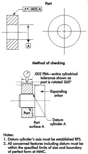
FIG. 55. Checking runout from an ID datum.

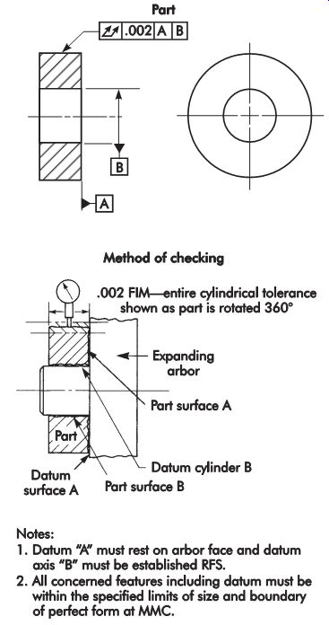
FIG. 56. Checking runout from a functional face and ID datums.

FIG. 57. Two parts with clearance holes assembled with bolts.

Substituting RFS for the MMC callout would make gaging difficult, if not impossible, since the gage pin must always be .01 in. (2.5 mm) smaller than the actual hole size. Eleven or more gage pins would be required for each hole (? .500 [12.70 mm]), ? .501 in. [12.73 mm], etc.). This is so that, for instance, if a particular hole measured ? .512 in. (13.00 mm), the ? .502 in. (12.75 mm) gage would be available for use.

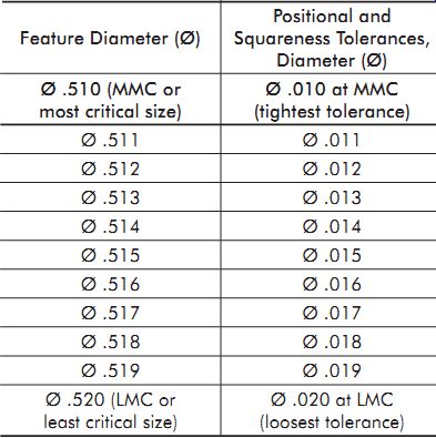
TBL. 2. Variable tolerances allowed by MMC

TBL. 2 shows how the true tolerance varies with hole size. All tolerances greater than ? .01 in. (2.5 mm) are bonus tolerances and not specifically allowed in any system other than the positional tolerancing system.

FIG. 58 shows the tolerances and gages for the manufacture and assembly of two different parts. One part contains clearance holes and the other holes are tapped for ? .50 in. (12.7 mm)

bolts. Also shown is the feature relation gage required for the tapped part. Gage thickness or bushing height must be at least the maximum thickness of the untapped part to guarantee the bolts will be properly located and square for assembly. The two go-thread gages simulate the bolts at assembly. Gage bushing size is determined by adding the ? .01 in. (2.5 mm) positional tolerance specified for the tapped features to the bolt or tap size. Stepped gage pins with go threads may be used to take advantage of standard bushing size as long as .01 in. (2.5 mm) difference in size is maintained between the gage bushing and that portion of the gage pin that lies within the bushing.

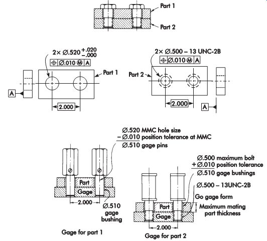
FIG. 58. Tolerances and gages for the manufacture and assembly of two different parts.

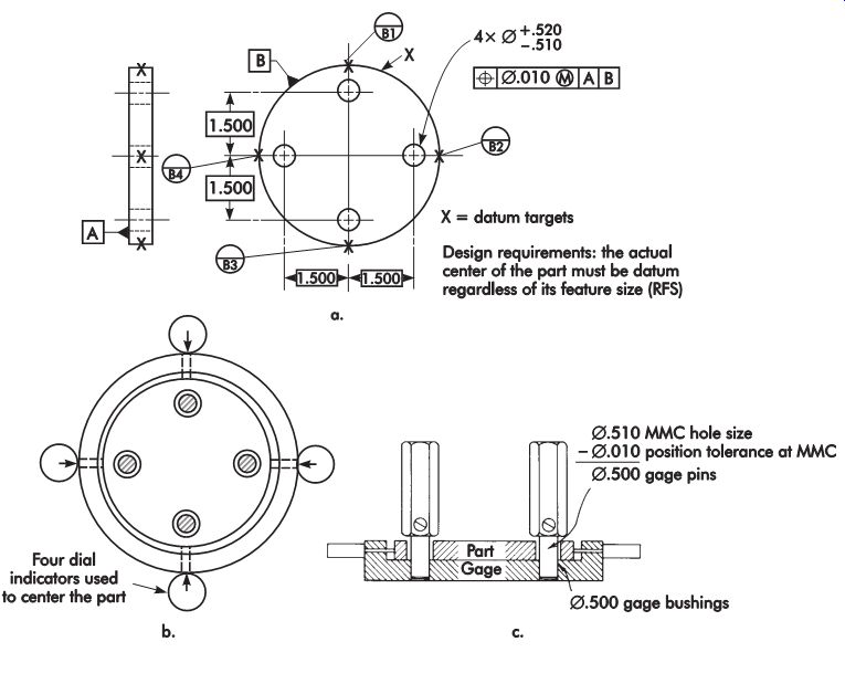
FIG. 59. Workpiece with four holes that must be located from the specific center of the workpiece.

Design Rules For Positionally Toleranced Parts

Two basic rules govern the design of gages for positionally toleranced parts. These principles apply regardless of the number of features that make up an interchangeable pattern.

1. For parts with internal features, the nominal gage feature size is directly determined by subtracting the total positional tolerance specified at MMC from the specified MMC size of the feature to be gaged for location.

2. For parts with external features, the nominal gage feature size is directly determined by adding the total positional tolerance specified at MMC to the specified MMC size of the feature to be gaged for location.

FIG. 59 shows a workpiece with four holes that must be located from the specific center (datum) of the workpiece regardless of the actual workpiece size (RFS). The design specification drawing includes the exact pickup points so the same center can be repeatedly found. Also shown is a hole relation gage that uses four dial indicators to determine and correctly position the datum for the hole-gaging operation.

FIG. 60 shows a similar workpiece with the less critical MMC requirement on the datum diameter. The holes are located from the center of the datum diameter when the datum is at MMC. Also shown is the design of a gage to check the part functionally.

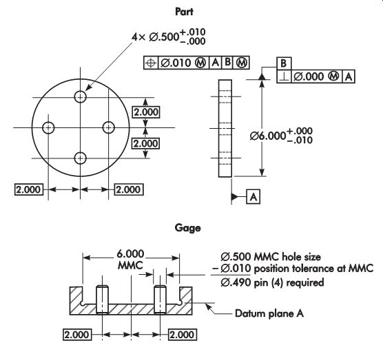
FIG. 60. "Shake" gage to check a less critical (MMC) OD datum feature.

FIG. 61 shows another workpiece in which the holes never need to be exactly located from the center of a specified datum feature. A gage-fit allowance has been specified. It is directly reflected in the size of the datum gage feature since the gage is ? .995 in. (25.27 mm) and differs from the MMC size of the part (? 1.000 in. [25.40 mm]) by .005 in. (0.13 mm). A fairly large allowance could be specified if the datum was merely a convenient starting place for manufacturing.

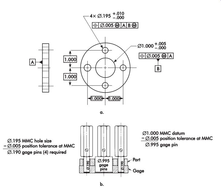
FIG. 61. Gaging workpiece features not specifically located relative to the datum: (a) workpiece; (b) hole location (shake) gage.

A pattern of interchangeable features (holes) is the most critical feature on the part shown in FIG. 62, but it is not locationally critical in relation to any single datum feature. The .30 in. (7.6 mm) minimum breakout specification is the result of a stress analysis and an end-product requirement. No single datum is specified, and the .30 in. (7.6 mm) minimum specification can be readily gaged with a tubing micrometer or a fork gage as shown.

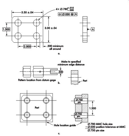
FIG. 62. Gaging an end product: (a) workpiece; (b) gage for checking required edge distance; (c) gage for checking hole location.

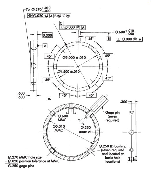
FIG. 63. Gaging radial hole patterns: (a) workpiece; (b) hole location and squareness gage.

FIG. 63 shows a workpiece with seven holes. The specified positional tolerance includes the location and angularity tolerances for each radial hole. Also shown is the gage required for checking the part. In use, all seven gage pins must go through the part at one time. In designating the datum, if RFS callouts had been used instead of MMC for the diameter and width of the slot, the gage would be required to center on the two datum features. As a result, one gage pin could be used to individually qualify each hole in Reference to the datum.

Position tolerance is often used to control the location of coaxial mating part features, as shown in FIG. 64, along with the gages to check them.

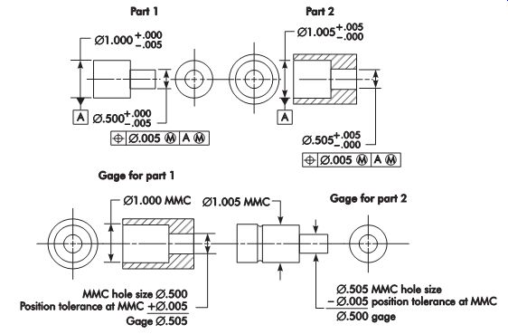
FIG. 64. Gaging coaxial mating parts at MMC.

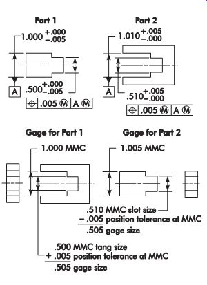
FIG. 66. Checking non-cylindrical mating parts at MMC.

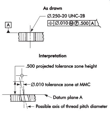
FIG. 67. Projected tolerance zone.

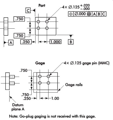
FIG. 68. Positional tolerance of zero at MMC.

FIG. 65 shows the method used to check bore alignment functionally when specified at MMC. Another common application of position tolerance at MMC is on non-cylindrical mating parts, such as those shown in FIG. 66. Occasionally, a projected tolerance zone will be specified to prevent interference at assembly, as shown in FIG. 67, along with its interpretation.

A case where it was desired to place all the usable size and location tolerances into the size limit by stating the position tolerance as zero (.000) at MMC is shown in FIG. 68, along with the functional gage to check the part. It should be noted that the gage eliminates the need for a go-plug-gage check.

Concentricity

Since concentricity tolerance is always on an RFS basis, it requires that the datum axis be established by chuck-like devices that close in on the part, or by electronic means previously described under runout. The latter allows the part to be mounted in any suitable fashion while indicating the datums and the features to be checked. Results are electronically interpreted and any eccentricity is displayed directly on the readout. All features must be measured separately to ensure that the part conforms to specified size tolerances.

Symmetry

Symmetry tolerances will be specified on non cylindrical parts on an RFS basis. Symmetry can be checked with standard surface-plate methods. However, for high production the multi-sensor-type electronic gaging methods mentioned previously for checking other RFS features are recommended.

References

ANSI B4.4M-1981 (R1994). Inspection of Work pieces. Washington, D.C.: American National Standards Institute.

ANSI/IEEE 268-1992. Metric Practice. Washington, D.C.: American National Standards Institute.

ASME B1.2-1983 (R2007). Gages and Gaging for Unified Inch Screw Threads. New York: American Society of Mechanical Engineers.

ASME B4.2-1978 (R2004). Preferred Metric Limits and Fits. New York: American Society of Mechanical Engineers.

ASME B46.1-2002. Surface Texture (Surface Roughness, Waviness, and Lay). New York: American Society of Mechanical Engineers.

ASME B5.10-1994. Machine Tapers-Self-holding and Steep Taper Series. New York: American Society of Mechanical Engineers.

ASME B89.3.1-1972 (R2003). Measurement of Out-of-roundness. New York: American Society of Mechanical Engineers.

ASME B94.11M-1993 (R1999). Twist Drills. New York: American Society of Mechanical Engineers.

ASME B94.6-1984 (R2009). Knurling. New York: American Society of Mechanical Engineers.

ASME Y14.1-1995 (R2005). Decimal Inch Drawing Sheet Size and Format. New York: American Society of Mechanical Engineers.

ASME Y14.2M-1992 (R2003). Line Conventions and Lettering. New York: American Society of Mechanical Engineers.

ASME Y14.3M-2003. Multiview and Sectional View Drawings. New York: American Society of Mechanical Engineers.

ASME Y14.36M-1996 (R2008). Surface Texture Symbols. New York: American Society of Mechanical Engineers.

ASME Y14.38-2007. Abbreviations and Acronyms Revision and Re-designation of ASME Y1.1-1989.

New York: American Society of Mechanical Engineers.

ASME Y14.5.1M-1994 (R2004). Mathematical Definition of Dimensioning and Tolerancing Principles. New York: American Society of Mechanical Engineers.

ASME Y14.6-2001 (R2007). Screw Thread Representation. New York: American Society of Mechanical Engineers.

ASME Y14.6aM-1981 (R1998). Screw Thread Representation (Metric Supplement). New York: American Society of Mechanical Engineers.

ASME Y14.7.1-1971 (R2003). Gear Drawing Standards-Part 1: For Spur, Helical, Double Helical, and Rack. New York: American Society of Mechanical Engineers.

ASME Y14.7.2-1978 (R1994). Gear and Spline Drawing Standards-Part 2: Bevel and Hypoid Gears. New York: American Society of Mechanical Engineers.

ASME Y14.8M-1996 (R2002). Castings and Forgings. New York: American Society of Mechanical Engineers.

Other Refs.

The Society of Manufacturing Engineers (SME) has developed the Fundamentals of Tool Design video series, which comprises nine DVDs, of which one relates directly to this section's content: Gaging & Inspection Tool Design (19 minutes).

Because of the limits of manufacturing, all nominal part dimensions require working tolerances for production. This program examines the variety of gaging tools used to determine if parts fall within their specified tolerances ranges.

These tools include screw-pitch gages, plug gages, ring gages, and snap gages.

Also examined are the various types of tools and systems used to amplify or magnify dimensions for measurement, including dial indicators, electronic digital readout, air gaging, coordinate measurement systems, optical projection, non contact sensor systems, and vision systems.

QUIZ

1. Define "tolerance."

2. Convert a bilateral tolerance of ±.007 in. (±0.18 mm) to a tolerance of position.

3. Convert a tolerance of position of .014 in. (0.36 mm) diameter to a bilateral tolerance.

4. Using the unilateral system of tolerancing, specify the correct nominal sizes and the gagemaker's tolerance to be applied for go and no-go working ring gages to check a shaft with a diameter of .8805 in. ±.0003 in. (22.4 mm ±0.008 mm). Include 5% wear allowance.

5. What bilateral tolerance would be applied to a master gage used to set a working gage measuring a dimension with a tolerance of ±.002 in. (±0.05 mm)?

6. Why is the unilateral system of gage-tolerance allocation preferred over the other systems?

7. What is the largest specimen diameter that could be completely viewed on a 30 in. (762 mm) optical comparator at 10× magnification? at 20×? at 31-1/4×? at 50×? at 62 1/2×? At 100×?

8. What gage material is used for a medium size production run? For higher-volume production? For situations requiring high accuracy or high wear?

9. What are the materials most used for surface plates?

10. What are the limitations of a screw-pitch gage?

11. What is the most widely used instrument for precise measurement?

12. What is the meaning of FIM?

13. What are the basic elements of electronic gages?

14. What are the two most common structural configurations for CMMs?

15. What is the primary application of optical flats?

16. Define "allowance" as it pertains to gages.

17. Define the following classes of tolerance fits:

a. running or sliding fit (clearance fit)

b. transition fit

c. force or shrink fit (interference fit)

18. What is the usual standard tolerance on tool dimensions if not otherwise specified? Indicate the standard tolerance for fractional, decimal-inch, and metric dimensions.

19. A .5-in. (12.7-mm) nominal sized shaft is to have an FN1 press fit. Calculate the tolerance for the hole and shaft and determine the limits of interference at the maximum material condition (MMC).

Home  PREV.  NEXT  Article Index  top of page