AMAZON multi-meters discounts AMAZON oscilloscope discounts
(cont. from part 1)
12. ENERGY IN ELECTRIC CIRCUITS
Because energy = power × time, the amount of energy used is directly proportional to both the power of a system and the length of time it is in operation. Because power is expressed in watts or kilo watts and time in hours (seconds and minutes are too small for practical use), the units of energy used are watt-hours (Wh) or kilowatt-hours (kWh).
EXAMPLE 7 (a)
Find the daily energy consumption of the appliances listed if they are used for the length of time shown.
Toaster (1340 W) Percolator (500 W) Fryer (1560 W) Iron (1400 W) 15 min 2 h
½ h
½ h (b)
Assuming that the average cost of energy is $0.12 per kilowatt-hour, find the daily operating cost.
SOLUTION
(a) Toaster:
Percolator:
Fryer:
Iron:
Total 1340 W = 1.34 kW × ¼ h
= 0.335 kWh 500 W = 0.5 kW × 2 h
= 1.00 kWh 1560 W = 1.56 kW × ½ h
= 0.78 kWh 1400 W = 1.4 kW × ½ h
= 0.70 kWh
2.815 kWh per day (b)
The daily operating cost is 2.815 kWh × $0.12/ kWh = $0.3378 (say, 34 cents).
The power used by a residential household varies with the time of day. A graph showing the power used by a typical American household during a normal weekday might look something like the one in Fig. 12. The average power demand of the household is much lower than the maximum.
The ratio between the two is called the overall load factor and runs between 20% and 30% for a typical household. The energy used by this household for the 24-hour period is represented by the area under the curve of Fig. 12. This can be determined only by integration because it varies continuously. Such integration is exactly what a kilowatt-hour meter does, as explained in Section 15 (dealing with electrical measurements).
EXAMPLE 8 It has been estimated that the aver age power demand of an American household with an electric stove is 1.8 kW. Calculate the monthly electric bill of such a household, assuming a flat rate of $0.12 per kilowatt-hour.
SOLUTION
Monthly energy use:
1.8 kW 24 h day 30 days month 1296 kWh per month ×× =
Monthly electric bill:
1296 kWh × $0.12/kWh = $155.52 ¦
In Example 25.8 the bill was based on a flat rate of 12 cents per kWh. Flat rates are very common for residential users. In the United States, residential rates vary from a low of 5-6 cents per kWh in states using substantial hydroelectric power to as high as 17 cents per kWh in some Northeastern states.
Hawaii has the highest rates in the United States.
Electric utilities (by franchise agreement) must provide for a customer's maximum power demand, whereas the monthly energy billing only compensates them for average demand, which is always lower. One technique used by electric utilities to account for this condition is to levy a demand charge for short-term power (kW) requirements in addition to the normal energy (kWh) billing for overall consumption. This technique has long been standard for industrial and commercial user rates, but it is still unusual for residential users. The demand charge is especially useful as a means of encouraging users to reduce their peak loads. In so doing, energy use is also somewhat reduced. As utilities continue to adjust to deregulation and rapidly fluctuating fuel costs, and incur difficulties meeting growing demands for service, expect to see more innovative (and complex) billing schemes being implemented.
13. ELECTRIC DEMAND CHARGES
Electric utility companies normally levy a kW demand charge on all but individual residential and a few special-category customers. Varying with the utility company involved, this monthly charge runs between $2 and $15 per kW of maximum average demand in any demand interval for a given month.
Demand intervals vary, usually being either 15 or 30 minutes (see Fig. 13).
Many utilities use a sliding window interval timing technique that starts a new interval every minute and updates the maximum interval demand accordingly. This enables them to find and bill for the maximum electric power demand in any 15- or 30-minute period in a month. Some companies also include a ratchet clause that levies a demand charge for a number of months based upon the maximum demand in any single month. This penalizes users with seasonal highs-that is, users with a low yearly load factor. The load factor is a measure of uniformity of power demand; a low load factor indicates short-time demand peaks for which the user is heavily charged. The justification for the imposition of a demand charge and the significance of load factors can best be demonstrated by an example.
Assume that a pottery manufacturer, whose average 8-hour daily load is 20 kW for lighting and pottery wheels, operates two 50-kW electric kilns twice a month for a 4-hour period each time. Further assume an energy charge of $0.10 per kWh.
The total monthly energy bill for the operation of the two kilns would be energy cost 2 50 kW 8 h
$0.10 kWh
$80.00 =× × × =
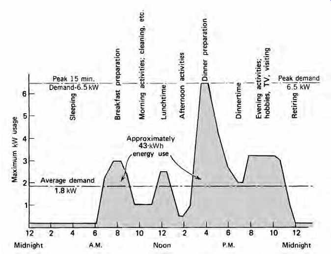
Fig. 12 Hypothetical graph of power usage for a typical U.S. household.
Electric cooking is assumed. The area under the curve represents energy usage.
Maximum kW demand (vertical axis) is based on a 15-minute integrated demand,
thus eliminating spikes in demand, such as those caused by starting a refrigeration
(air-conditioning) compressor. This curve has a 24-hour use of approximately
43 kWh, giving an average 24-hour demand of 1.8 kW. The ratio between this
average demand and the peak demand of 6.5 kW is called the load factor, which
here is 27.5%.
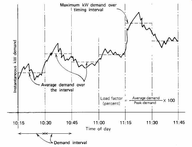
Fig. 13 Typical instantaneous load curve for a commercial facility. The
utility demand meter records the average demand in each period (here, 15 minutes).
The maximum interval demand-in this case, between 11:15 and 11:30-is used as
the basis for monthly billing. A high load factor (utilization factor) indicates
that little can be gained by demand control; a low load factor indicates the
reverse.
Thus, were it not for a demand charge, the utility company, which is required by law to supply the maximum customer demand, would have to pro vide and maintain 100 kW of generation, trans mission, and distribution facilities in return for a payment that is the equivalent of 1.11 kW of aver age continuous load, that is, equivalent continuous load
$80.00 720 hr/mon
=
t th 0.10 ×
= 1.11 kW The user's load factor can be calculated readily. By definition, load factor average power demand maximum power d
=
e emand
(25.8)
For a given time interval (e.g., day, month, year), the average power demand is equal to the energy used in the period divided by the period length.
Average period power demand
=
kWh energy use hours of use for that time period d (25.9)
Therefore, the average monthly power demand equals the average monthly energy use divided by 720 hours. Substituting the monthly version of Equation 25.9 as the general expression for the load factor (LF) in Equation 25.8 gives LF monthly
=
÷ monthly kWh energy use 720 hours maximum demand
(25.10)
For the case under consideration, the monthly load factor is LF (2 days 4 h 100 kW)] 720 h 120 kW
=
+×× ÷
[ [(23days 8h 20kW) ××
=
+÷ (3680 800 kWh/month) 720 h 120 kW
= 0.052 or 5.2%
This is a very poor load factor, which results in the levying of a high demand charge. Assuming an $8.00 per kW demand tariff, this pottery manufacturer would be billed, monthly, an additional demand charge = 120 kW × $8.00 = $960.00
With an energy bill of only energy cost = 4480 kWh × $0.10 = $448.00 this manufacturer is paying heavily for high peak power use.
Although the illustration selected is somewhat extreme in its pattern of electricity use, it is not uncommon to find demand charges of the same order of magnitude as energy charges. It is impossible to eliminate demand charges entirely, but it is certainly possible (and frequently very simple) to reduce them. Such reduction is in the interest of the user, the utility, and the public at large: the user- for economic reasons; the utility-to permit more efficient use of its facilities; and the general public- by avoiding unnecessary power plant construction and associated inefficient use of fuel during partial generator loading, and by overall reduction in fuel use. The last item is a secondary benefit of demand control.
The next section discusses user electric demand control, the primary function of which is to reduce electric power demand. This reduces demand charges and, incidentally (secondarily), somewhat reduces energy consumption. Electric demand control is different from energy management, which is primarily concerned with reduction of all types of energy use, including electricity. Electric demand control is frequently included as one part of an over all energy management system.
14. ELECTRIC DEMAND CONTROL
Electric demand control methods vary greatly in complexity and in degree of automation, but all basically perform the same task-enabling efficient utilization of available energy to produce a high load factor, resulting in a lowering of demand charges.
An ancillary but important benefit is the improved utilization of building electrical power equipment, which normally runs underloaded. When demand control is incorporated during the original design (instead of as a retrofit), it results in smaller equipment, a lower first cost, and less space allocated for equipment.
For a number of years beginning in the 1980s, many utilities offered their customers rebates that covered up to 40% of the cost of equipment and renovations that would reduce maximum demand and overall energy use. These programs acted as a clear financial incentive for the development of cost-effective demand control and energy conservation equipment and techniques that have since become widely adopted. The result has been a considerable reduction in nationwide per capita electric power and energy use. These rebate programs reduced the investment payback period to such an extent that many (perhaps most) large power users invested large sums in electric demand control and energy conservation and management equipment.
The advantage to the energy user is obvious: lower electric bills. The advantage to the utility is equally simple. It costs $3500 to $5000 per kilo watt of generating capacity for new power plant construction (depending upon the location and required auxiliary construction), whereas rebates run from $150 to $1000 per kW conserved, with the larger amounts paid for by peak demand reduction. Because a utility must supply all the power demanded by customers, it is very much in the interest of any utility that is generating power output near the maximum capacity of its equipment to reduce loads in general and peak loads in particular.
The oldest and simplest utility-sponsored demand control scheme, still in use today, is the time-of-day-dependent, variable utility rate schedule. This scheme encourages off-peak use of electricity by offering a lower energy rate for consumption during off-peak hours. Utilities offering off-peak rates generally install, at no charge to the user, a separate time-controlled circuit switch for use with time-deferrable loads such as water heaters, well pumps, battery chargers, and the like. The circuit is energized only during off-peak hours, which typically are mid-afternoon and after midnight. One such arrangement is shown in Fig. 14. Note that the switch itself has no programming buttons. All programming is done by the utility with an auxiliary programmer (shown) that can be used to pro gram many user switches.
The basic technique of user demand control is simple; electric loads are disconnected and reconnected in such a fashion that demand peaks are leveled off and the load factor is thereby improved.
The extent to which a user's electric loads can tolerate this type of switching is an indication of the potential effectiveness of a demand controller. An installation with a large uninterruptible load, such as from computers or other productivity equipment, benefits minimally from demand control.
Most industrial and commercial installations, however, contain a large percentage of interruptible loads (interruptions may be very short), and demand control systems frequently accomplish a 15% to 20% reduction in electric bills with a resultant short payback period on equipment investment.
The proliferation of demand control equipment has also produced a proliferation of nomenclature, including load shedding control, automated load control, peak demand control, and programmable load control. Descriptions that include the term energy management refer to devices whose primary function is the control of energy consumption and that secondarily are equipped to provide electric demand control.
Demand control devices are intended to control power, which is timed energy use. Demand control produces energy savings as a secondary benefit.
The expression electric demand control is used for simplicity in the following sections. Various demand control schemes are discussed in some detail to enable the reader to differentiate them by recognizing their specific characteristics. Much equipment on the market today provides additional functions not directly related to demand control. Thus, a good understanding of the essentials of demand control schemes will greatly assist the prospective user. As with other areas of design, manufacturers' literature usually comprises a lengthy list of equipment abilities, few (if any) shortcomings, and little indication of specific or comparative applicability.
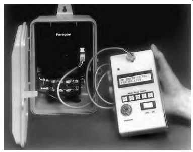
Fig. 14 Programmable electronic time control switch designed for time-of-use
(off-peak) utility rate schedules. The programming device is separate from
the switch and can be used by a utility to program many customer switches.
The illustrated unit is arranged for 365-day scheduling, which permits full
coordination with utility schedules that vary with the seasons of the year.
Typical controlled loads include water heaters, thermal storage units, water
and air accumulators, and any other load that either inherently or by design
can be delayed for several hours. (Courtesy of Paragon Electric Co., Inc.)
(a) Level 1-Load Scheduling and Duty-Cycle Control
This level is the simplest and most direct approach, and is applicable to all types of facilities. A facility's electric loads are analyzed and scheduled to restrict demand. Accordingly, large loads can be shifted to off-peak hours and controlled to avoid coincident operation. The scheduling can take advantage of special night and weekend utility rates for loads (such as battery charging and transfer pumping) that do not require a specific time of operation. The demand control device used is essentially a programmable time switch (see Section 26) applied to a number of circuits or loads. It is not, strictly speaking, a demand controller, in that no real-time measurement is made of the actual continuous electric load. Instead, the control operates on a preset timed duty cycle relying entirely on a prior analysis of the building loads. Typical applications of this device are control of HVAC loads, lighting loads, and pro cess loads in small commercial, institutional, and industrial buildings.
(b) Level 2-Demand Metering Alarm
If, in conjunction with a duty-cycle controller, some type of continuous demand metering is installed that goes into alarm mode when a predetermined demand level is exceeded, a basic load (demand) control system will have been established. The load analysis discussed previously would be structured and used to determine load priorities so that when a preset maximum demand load is exceeded and the alarm sounds, loads can be shed (disconnected) manually in a pre-established order of priority-and subsequently reconnected, also in order of priority.
This type of control is practical only for a moderate size installation, inasmuch as the load-switching activity is manual.
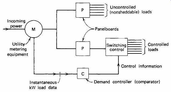
Fig. 15 Block diagram of a system for automatic electric power demand
control. The demand controller receives instantaneous load data from the metering
equipment, compares them to preset limits, and disconnects and reconnects controllable
loads automatically to keep kW demand (load) within these limits.
(c) Level 3-Automatic Instantaneous Demand Control This type of control (also called rate control) is, in effect, an automated version of the level 2 system described in the preceding subsection. The control unit accepts instantaneous kilowatt load information from the utility system, compares this information to a preset kilowatt limit, and acts automatically to disconnect and reconnect loads as required. These units do not recognize the utility's metering interval but act continuously on the basis of load comparison data. For this reason, these units are also referred to as load comparator controllers.
Figure 15 will help explain the unit's operation.
Typical sheddable loads might include nonessential lighting, some cooling load, domestic hot water heating, snow melting, and the like. Non sheddable loads (that do not tolerate even short interruption) might include essential lighting, elevators, communications equipment, computers, process control, emergency equipment, and the like. The nonsheddable loads are fed directly from the power line. The sheddable loads are fed through a panel of control relays that respond to on/off instructions from the demand controller. Although the resulting energy use with or without the controller is theoretically the same, in practice energy savings of 15% and more are common.
The principal drawback of this system is that the load shedding is preprogrammed. This results in an inability to readily adapt to varying load pat terns resulting from variable production schedules, time schedules, changes in weather, and so on. As a result of this limitation, this system is most useful in applications where operating modes do not change frequently and the facility is not very large. Thus, stores, supermarkets, warehouses, small industrial facilities, and commercial installations are well served with this type of system if they have at least 20% sheddable loads and their connected electric load is at least 150 kilovolt-amperes (kVA).
This level of demand control, as well as levels 4 and 5 described later, is most often supplied as one of many functions of a larger building energy control system. Because this is so, it is necessary to ascertain that the type of demand control to be supplied by the overall building control hardware and software is what the electrical system designer intended.
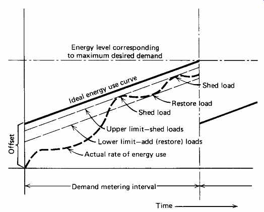
Fig. 16 Graph of the action of an ideal rate controller. Note that toward
the latter part of the period the pattern has been established, and the actual
rate of energy use corresponds closely to the ideal. This type of control is
often simply a part of the software in a large, centralized building control
system.
(d) Level 4-Ideal Curve Control
This control function operates by comparing the actual rate of energy usage to an ideal rate and controlling kilowatt demand by adjusting the total energy used within a metering interval. The utility company determines the demand over the demand interval by integrating the kilowatt-hour energy consumption over the interval and dividing by the interval time. Thus, the user is actually given a block of energy (kWh) that can be utilized at any desired rate, not necessarily at a constant rate. The desirable rate of energy use is shown as the "ideal curve" on the typical usage curve shown in Fig. 16.
Shed points can be programmed independently for each load according to a predetermined priority, and priorities can be readily adjusted and rescheduled. Loads are normally shed only toward the end of an interval-when the permissible energy total for the interval is approached-and all loads are restored at the beginning of the next interval. Thus, during each interval, sheddable loads are off for only a few minutes at most. Controllers operating on the ideal curve principle are considerably more flexible than the kilowatt rate controller described in the level 3 system, and are applicable to facilities of widely divergent load size, but with at least a 300-kW connected load. As with other controllers, the principal savings will be in demand charges, but almost always with considerable savings in energy billings.
(e) Level 5-Forecasting Systems
These systems are by far the most sophisticated, the most expensive, and the most effective. They are best applied to large facilities where the number of loads, load patterns, and complexity of operation preclude the effective use of the preceding systems.
Because of the large amount of load data that needs to be processed, these systems are usually installed as part of a computerized central control system.
Details of operation are too complex to be described here, but the basic operation can be outlined. These control units operate by continuously forecasting the amount of "unpenalized" energy remaining in the demand interval, based upon kilowatt-hour data received. They then examine the status and priority of each of the connected loads and decide on a course of action. Loads that in other systems are classified as nonsheddable are, in this system, controlled because of the accuracy and rapidity of the control function. A pneumatic compressor, for instance, that supplies process air might, in lower level control systems, be classified as non-controllable, despite the fact that it has long off periods. With computer control, such a load would be classified as "delayable" or "inhibited" because a 30-second or 1-minute delay in activation after the pressure switch closes its contact is normally acceptable.
The advantage of these systems is that, if programmed properly, they can make small, accurate load changes throughout an interval, resulting in minimum load cycling and maximum efficiency.
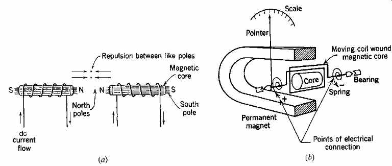
Fig. 17 (a) Diagram showing the basic electromagnetic principle and interaction
between electromagnets. Any iron core becomes an electromagnet when current
flows in a coil wound around it, as shown. (b) The principle of the electromagnet
is used in this basic meter movement. Current flowing in the movable coil forms
an electromagnet whose field interacts (see a) with the permanent mag net's
field, causing a deflection proportional to the current flow. (Courtesy of
Wechsler, a division of Hughes Corp.)
15. ELECTRICAL MEASUREMENTS
The preceding sections have explained the fundamental electric quantities of voltage and current and defined the units involved as volts and amperes, respectively. As is true of all physical quantities used in practical applications, a need exists for a simple means of measuring these quantities. This need was initially met by the development of the meter movement illustrated in Fig. 17.
Everyone at one time or another has felt the repulsion between like poles of two magnets held close together and, conversely, the attraction between opposite poles. This principle was used in the first basic meter movement: causing a deflection of the pointer as a result of the repulsion between the field of a permanent magnet and an electromagnet. The electromagnet is formed when current flows in the coil, and its strength is proportional to the amount of current. Thus, a strong current causes a larger deflection of the needle and therefore a higher reading on the dial. A spring (see Fig. 17b) provides restraining torque on the pointer. To make this very sensitive unit usable for large currents (it is intrinsically a micro-ammeter, sensitive to millionths of an ampere), the device simply diverts, or shunts away, most of the current, allowing only a few microamperes to actually flow in the meter coil.
To use the same device as a voltmeter, a large resistance called a multiplier is placed in series with the meter, thereby again limiting the current flow to a few microamperes. The meter scale is then calibrated in volts. All dc meters are made in this fashion. Most ac meters operate on basically the same principle, except that instead of a permanent magnet, an electromagnet is used. Thus, when the polarity reverses, the deflecting force retains the same direction. A dc meter connected to an ac circuit simply will not read because inertia prevents the needle from bouncing up and down 60 times a second.
The meters just described are conventional analog devices that read electrical values in pro portion to mechanical forces exerted within the device-that is, by analogy. Modern electronics has produced a line of solid-state electrical meters (Fig. 18) that display the measured electrical values in analog mode (needle on a dial), digital mode, or both. They operate in a number of ways, all of which are different from that described previously and are beyond the scope of this book.
The fact that a meter reads digitally does not necessarily mean that it is highly accurate. Accuracy depends upon the quality of the internal circuitry. Digital meters are easier to read than analog meters because no visual interpretation or interpolation is involved. This advantage, plus the constantly declining cost of sophisticated electronics, will undoubtedly lead to solid-state digital meters replacing analog types, except for special applications.
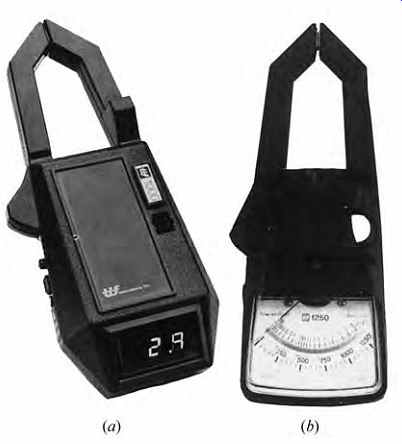
Fig. 18 (a) Solid-state clamp-on type meter with digital readout and automatic
ranging. The latter feature eliminates the necessity to preselect a meter range
and is particularly useful where the magnitude of current or voltage is unknown.
The clamp-on feature permits use without wiring into, or otherwise disturbing,
the circuit being measured. The meter measures approximately 8 × 3 × 1.5 in.
(200 × 75 × 40 mm), weighs less than 1 lb (0.5 kg), and is battery-powered.
Scales are 0.1-1000 amp ac, 0.1-1000 V ac, and 0.1-1000 ohms resistance, with
±2% accuracy. (b) Solid-state auto-ranging clamp-on ac meter with analog-type
readout. It is similar in design to the meter in (a), but with somewhat larger
range scales and additional features such as peak current measurement. (Photos
courtesy of TIF Instruments, Inc.)
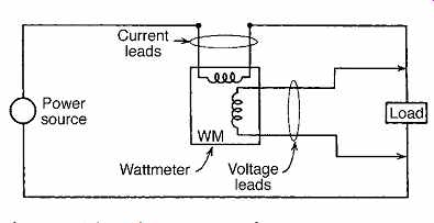
Fig. 19 Schematic arrangement of wattmeter connections. Note that the current
coil is in series with the circuit load, whereas the voltage leads are in parallel.
In buildings, the measurement of current and voltage is generally not as important as the measurement of power and energy. To measure power, the fact that power is proportional to the product of the voltage and current in a circuit is employed.
Although actual construction is complex, the theory of operation of a conventional coil-type wattmeter is simple. The meter has two coils: a current coil that is similar in connection to an ammeter and a voltage coil that is similar in connection to a voltmeter (Fig. 19). By means of the physical coil arrangement, the meter deflection is proportional to the product of the two and therefore to the circuit power. The meter can be calibrated as desired, depending upon the size of the shunts and multipliers.
To measure energy, the factor of time must be introduced because:
energy = power × time
Direct current energy meters are available but are not of general interest because of the rarity of dc power. Alternating current watt-hour meters are basically small motors, whose speed is proportional to the power being used. The number of rotations is counted on the dials, which are calibrated directly in kilowatt-hours. A diagram of the basic construction of an ac kilowatt-hour meter is shown in Fig. 20. As can be seen, kilowatt-hour energy consumption and maximum interval kilowatt demand can be read directly from the dials. If the numbers involved are too large (because of calibration), a multiplying factor is required to arrive at the proper kilowatt-hour consumption. This number is written directly on the meter nameplate, and the meter reading is multiplied by it to get the actual kilowatt hours. Several types of solid-state multifunction and energy meters are shown in Figs. 21, 22, and 23.
Continuous monitoring of the electrical characteristics of an entire distribution system, or of a portion fed from a specific switchboard, can be readily accomplished by use of the solid-state device shown in Fig. 24. This programmable analyzer can be arranged to measure power usage, perform power quality and harmonic analyses (and the like), and display the results locally and remotely.
Because manual reading of kilowatt-hour meters of individual consumers is a labor-intensive task-even without the routine job difficulties such as inaccessible meters, unfriendly dogs, inclement weather, and so on-utilities have long sought a more cost-effective means of determining consumer energy usage. To this end, with the benefit of modern microelectronics, a number of interesting, labor-saving kilowatt-hour meters have been developed. One type is equipped with a programmable electro-optical automatic meter reading system that can be activated locally or from a remote location. The meter data are transmitted electrically to a data-processing center, where they may be used by the utility to prepare subscribers' bills; prepare customer load profiles; and study, in combination with other data, area load patterns, equipment loadings, and so on. The customer can use instantaneous data to control loads, as explained in the preceding section.
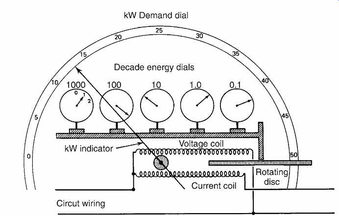
Fig. 20 Typical induction-type kilowatt-hour meter with kilowatt demand
dial. Dials register total disc revolutions, which are proportional to energy.
Disc rotational speed is proportional to power. Note that the current coil
is in series with the load and that the voltage coil is in parallel.

Fig. 21 (a) A modern multifunction solid-state kWh meter. This single-phase
meter includes a mechanical register similar to that shown in Fig. 20 plus
a large liquid crystal display. It can be arranged to provide either time-of-use
billing or demand/time-of-use billing in addition to its energy measurement
function. It can also be configured to provide load control, demand threshold
alert, end of-interval alert, and load profile recording. (b) Field programming
of the meter shown in (a) is accomplished with a hand-held programming device.
(Photos courtesy of Landis and Gyr.)
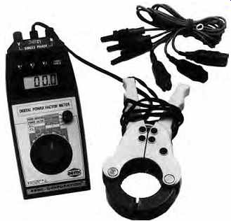
Fig. 22 Digital power factor meter, which measures the power factor on
single- and 3-phase circuits. In addition, the meter can measure 0-600 V ac
and 0-2000 A ac. Connections to the circuits being measured are made with the
clamp-on probes shown. A similar unit is available that measures power in both
sinusoidal and nonsinusoidal waveforms in the range 0.1 W through 2000 kW.
(Courtesy of AEMC Corporation.)
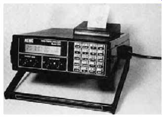
Fig. 23 This portable, programmable power analyzer unit measures approximately
13 × 7 × 12 in. (330 × 180 × 305 mm) and weighs 6 lb (2.7 kg). It is capable
of measuring (and computing) 19 electrical parameters, among which are current,
voltage, energy, power, power factor, and frequency, and of providing both
an instantaneous digital readout and printed records (hard copy). Connections
permit all functions to be addressed by remote control. (Courtesy of AEMC Corporation.)
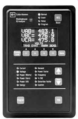
Fig. 24 Power system analysis unit designed to be mounted permanently into
a system switchboard (see Section 26). This programmable unit can meter circuit
parameters, measure energy and power use, analyze power quality (including
harmonic analysis), and log events. (Photo courtesy of Cutler Hammer.)
Another meter type is equipped with a miniature radio transmitter that can be remotely activated to transmit the current kilowatt-hour reading. The meter reader moves along a street and remotely activates a meter by entering a customer code into a digital pad. A special receiver not only receives the transmitted kilowatt-hour data but encodes and records the data automatically. These and other new kilowatt-hour meters are obviously much more costly than the traditional units, but they are gradually being introduced because of large reductions in labor costs and increases in the quantity and quality of data made available.
In this regard, programmable meters are currently being aggressively deployed among residential customers in some areas to allow utility company control of demand (with the agreement of the consumer-usually resulting from a more favorable rate structure).