AMAZON multi-meters discounts AMAZON oscilloscope discounts
Probabilistic thinking is based on very old ideas which go back to De Mere, La Place, and Bayes. What is probability and how does it relate to frequency, statistics and, finally, machinery reliability? The word probability has several meanings. At least three will be considered here.
One definition of probability has to do with the concept of equal likelihood. If a situation has N equally likely and mutually exclusive outcomes, and if n of these outcomes are event E, then the probability P_E_ of event E is:
P_E_ = n N
This probability can be calculated a priori and without doing experiments.
The example usually given is the throw of an unbiased die, which has six equally likely outcomes - the probability of throwing a one is 1:6.
Another example is the withdrawal of a ball from a bag containing four white balls and two red ones - the probability of picking a red one is 1:3. The concept of equal likelihood applies to the second example also, because, even though the likelihoods of picking a red ball and a white one are unequal, the likelihoods of withdrawing any individual ball are equal.
This definition of probability is often of limited usefulness in engineering because of the difficulty of defining situations with equally likely and mutually exclusive outcomes.
A second definition of probability is based on the concept of relative frequency. If an experiment is performed N times, and if event E occurs on n of these occasions, then the probability of P_E_ of event E is:
P_E_ = lim n?_
n N
P_E_ can only be determined by experiment. This definition is frequently used in engineering. In particular it’s this definition which is implied when we estimate the probability of failure from field failure data.
Thus, when we talk about the measurable results of probability experiments - such as rolling dies or counting the number of failures of a machinery component - we use the word "frequency." The discipline that deals with such measurements and their interpretation is called statistics.
When we discuss a state of knowledge, a degree of confidence, which we derive from statistical experiments, we use the term "probability." The science of such states of confidence, and how they in turn change with new information, is what is meant by "probability theory." The best definition of probability in our opinion was given by E. T. Jaynes of the University of California in 1960:
Probability theory is an extension of logic, which describes the inductive reasoning of an idealized being who represents degrees of plausibility by real numbers. The numerical value of any probability _A_B_ will in general depend not only on A and B, but also on the entire background of other propositions that this being is taking into account. A probability assignment is 'subjective' in the sense that it describes a state of knowledge rather than any property of the 'real' world. But it’s completely 'objective', in the sense that it’s independent of the personality of the user: two beings faced with the same total background and knowledge must assign the same probabilities.
Later, Warren Weaver [5] defined the difference between probability theory and statistics:
Probability theory computes the probability that 'future' (and hence presently unknown) samples out of a 'known' population turn out to have stated characteristics.
Statistics looks at a 'present' and hence 'known' sample taken out of an 'unknown' population, makes estimates of what the population may be, com pares the likelihood of various populations, and tells how confident you have a right to be about these estimates.
Stated still more compactly, probability argues from populations to samples, and statistics argues from samples to populations.
Whenever there is an event E which may have outcomes E1_ E2_____ En, and whose probabilities of occurrence are P1_P2_____ Pn, we can speak of the set of probability numbers as the "probability distribution" associated with the various ways in which the event may occur.
This is a very natural and sensible terminology , for it refers to the way in which the available supply of probability (namely unity) is "distributed" over the various things that may happen.
Consider the example of the tossing of six coins. If we want to know "how many heads there are," then the probability distribution can be shown as follows:
* No. of heads 0 1 2 3 4 5 6 Probability 1/64 6/64 15/64 20/64 15/64 6/64 1/64
These same facts could be depicted graphically ( Fig. 1). Accordingly, we arrive at a probability curve versus "frequency" as a way of expressing our state of knowledge.
As another application of the probability-of-frequency concept, consider the reliability of a specific machine or machinery system. In order to quantify reliability, frequency type numbers are usually introduced. These numbers are mean times between two failures or MTBF , for instance, which are based on failures per trial or per operating period. Usually they are referred to in months.
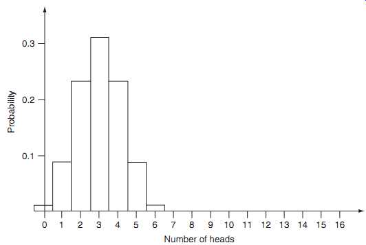
Fig. 1. Distribution of probabilities measured by the vertical height
as well as by areas of the rectangles (the six-coin case).
Most of the time we are uncertain about what the MTBF is. "All machines and their components are not created equal," their load-cycles and operating conditions are unknown, and maintenance attention can vary from neglect to too frequent intervention. Consider for instance the MTBF of a sleeve bearing of a crane trolley wheel. At a MTBF of 18 months (30% utilization factor), early failures can be experienced after 6 months. The longest life experience may be five times the shortest life (see Fig. 2). Even though the data were derived from actual field experience, we cannot expect exact duplication of the failure experience in the future. Therefore, Fig. 2 is our probabilistic model for the future of a similarly designed, operated, and maintained crane wheel.
It’s important to distinguish the above idea from the concept of "frequency of frequency." Let R denote the historical reliability of an individual designated machine, selected at random from a population of similar machines. The historical reliability of a machine is defined as:
R = 1- H1 H1 +H (3.3) where H1 = total time on forced outage _h_, H = total service time _h_.
We can build a frequency distribution using historical reliability for each machine showing what fraction of the population belongs to each reliability increment. If the population is large enough we can express this distribution as a continuous curve - a "frequency density" distribution,
__R_. The units of __R_ are consequently frequency per unit R, or fraction of population per unit reliability.
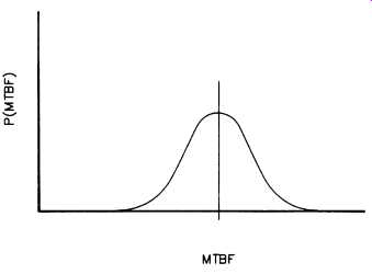
Fig. 2. Probability-of-frequency curve for a machinery component.
This curve is an experimental quantity. It portrays the variability of the population, which is a measurable quantity. The value of R varies with the individual selected. It’s a truly fluctuating or random variable.
Contrast this with the relationship shown in Fig. 2, where we selected a specific machinery component and asked what its future reliability would be. That future reliability is the result of an experiment to be done. It’s not a random variable: it’s a definite number not known at this time. This goes to show that we must distinguish between a frequency distribution expressing the variability of a random variable and a probability distribution representing our state of knowledge about a fixed variable.
A third definition of probability is degree of belief. It’s the numerical measure of the belief which a person has that an event will occur.
Often this corresponds to the relative frequency of the event. This need not always be so for several reasons. One is that the relative frequency data available to the individual may be limited or non-existent. Another is that although somebody has such data, he or she may have other information which causes doubt that the whole truth is available. There are many possible reasons for this.
Several branches of probability theory attempt to accommodate personal probability. These include ranking techniques, which give the numerical encoding of judgments on the probability ranking of items.
Bayesian methods allow probabilities to be modified in the light of additional information.
The key idea of the latter branch of probability theory is based on Bayes' Theorem, which is further defined below.
In basic probability theory, P_A_ is used to represent the probability of the occurrence of event A; similarly, P_B_ represents the probability of event B. To represent the joint probability of A and B, weuse P_A?B_, the probability of the occurrence of both event A and event B. Finally, the conditional probability, P_A_B_, is defined as the probability of event A, given that B has already occurred.
From a basic axiom of probability theory, the probability of the two simultaneous events A and B can be expressed by two products:
Equating the right sides of the two equations and dividing by P_B_, we have what is known as Bayes' Theorem:
In other words, it says that P_A_B_, the probability of A with information B already given, is the product of two factors: the probability of A prior to having information B, and the correction factor given in the brackets. Stated in general terms:
Posterior probability ? Prior probability × Likelihood where the symbol ? means "proportional to". This relationship has been formulated as follows:
_B_ is the posterior probability or the probability of Ai now that B is known. Note that the denominator of equation 3.7 is a normalizing factor for P_Ai
_B_ which ensures that the sum of P_Ai
_B_ = 1.
As powerful as it’s simple, this theorem shows us how our probability - that is, our state of confidence with respect to Ai - rationally changes upon getting a new piece of information. It’s the theorem we would use, for example, to evaluate the significance of a body of experience in the operation of a specific machine.
To illustrate the application of Bayes' Theorem let us consider some examples. If C represents the event that a certain pump is in hot oil service and G is the event that the pump has had its seals replaced during the last year, then P_G_C_ is the probability that the pump will have had its seals replaced some time during the last 3 years given that it’s actually in hot oil service. Similarly, P_C_G_ is the probability that a pump did have its seals replaced within the last 3 years given that the pump is in hot oil service. Clearly there is a big difference between the events to which these two conditional probabilities refer. One could use equation 3.6 to relate such pairs of conditional probabilities.
Although there is no question as to the validity of the equation, there is some question as to its applicability. This is due to the fact that it involves a "backward" sort of reasoning -- namely, reasoning from effect to cause.
Example: In a large plant, records show that 70% of the bearing vibration checks are performed by the operators and the rest by central inspection. Furthermore, the records show that the operators detect a problem 3% of the time while the entire force (operators and central inspectors) detect a problem 2.7% of the time. What is the probability that a problem bearing, checked by the entire force, was inspected by an operator? If we let A denote the event that a problem bearing is detected and B denote the event that the inspection was made by an operator, the above information can be expressed by writing:
P_B_ = 0 70, P_A_B_ = 0 03, and P_A_ = 0 027, so that substitution into Bayes' formula yields:
This is the probability that the inspection was made by an operator given that a problem bearing was found.
According to the foregoing, our understanding of reliability here is a probability rather than merely a historical value. It’s statistical rather than individual.