AMAZON multi-meters discounts AMAZON oscilloscope discounts
The reliability of a machinery system may be mathematically described by defining distribution functions using discrete and random variables.
An example of a discrete variable is the number of failures in a given time interval. Examples of continuous random variables are the time from part installation to failure or the time between successive equipment failures.
This approach has been particularly useful in the field of electronic engineering where it has been applied to the design and evaluation of electronic devices. Using reliability theory one can estimate the reliability of complex electronic systems. Calculation methods, specific to electronic systems, make use of failure probability data compiled for this purpose.
To evaluate electronic component reliability, the concept of constant failure rate is used, that is failure rates of electronic components remain constant during the useful life of the component. However, this is frequently not the case when evaluating mechanical component reliability.
There are several reasons for this. It is , for example, an established fact that in many cases machinery components follow an increasing failure rate pattern. Another reason is the fact that machinery components are not well standardized. Finally, there seem to be many more failure modes experienced by machinery parts than by electronic parts. Consequently, reliability data for mechanical components and assemblies is scarce, and, when available, caution is advised. From this it follows that there is no accurate method available for absolute reliability prediction that takes the specific nature of machinery systems into account. As we will see later, it seems that only relative reliability predictions can be made for machinery. What is the specific nature of machinery? Fig. 1 illustrates a machinery system by comparing it with an electric system. Consider , for example, the reliability of a tribo-mechanical system* in which wear behavior is a function of time. Three main characteristics may be deter mined for the loss-output wear rates of such a system:
1. Self-accommodation ("running-in")
2. Steady-state
3. Self-acceleration ("catastrophic damage")
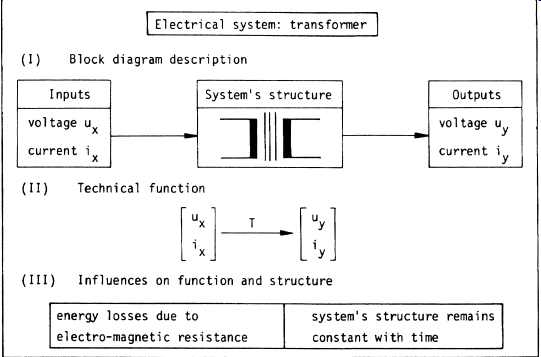
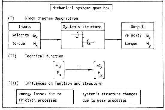
Fig. 1. Comparison of the characteristics of an electrical and a
mechanical system. (Czichos, H., Tribology--A
Systems Approach to the Science and Technology of Friction, Lubrication,
and Wear, 1978, p.
26, Fig. 1, Elsevier Science Publishers, Physical Sciences & Engineering
Div.)
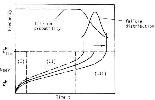
Fig. 2. Wear curves and failure distribution.
These three phase changes in the system behavior may follow each other in time ( Fig. 2). Here, ZM lim denotes a maximum allowable level of wear loss. At this level the system structure has changed in such a way that the functional input-output relationship of the system has been severely disturbed. Repeated measurements show random data variations as indicated by the dashed lines in Fig. 2. A distribution of the "life" of the system or a failure distribution can be derived from sample functions of the wear process.
Earlier, we familiarized ourselves with the concept of relative frequency. The reader is referred to Fig. 2, which for convenience, is reproduced in Fig. 3. If we wish to determine the probability of failure occurring between the times tb and tc, we multiply the y-axis value by the interval _tc -tb_. Fig. 3 is also called a probability density function where the equation of the curve is denoted by f_t_. As an exam ple, if f_t_ = 0_6 exp_-0_6t_, we obtain the curve shown in Fig. 4, a negative exponential distribution which will be dealt with later.
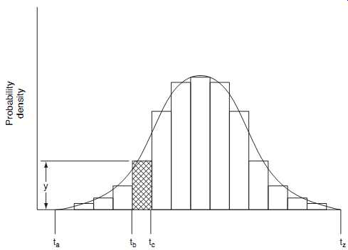
Fig. 3. Probability density function.
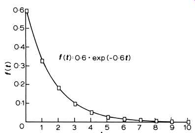
Fig. 4. Negative exponential distribution.
Returning to Fig. 3, the probability of a failure occurring between tb and tc is the area of the hatched portion of the distribution. This area is the integral between tb and tc of f_t_ or:
tc tb f_t_dt
Consequently, the probability of a failure occurring between times ta and tz is:
tz ta f_t_dt = 1
We stated earlier that the failure distributions of different types of machinery systems are not the same. Even the failure distributions of identical machines may not be the same if they are subjected to different levels of Force, Reactive Environment, Temperature, and Time (FRETT).
There are a number of well-known probability density functions which have been found in practice to describe the failure characteristics of machinery (see Fig. 5).
The cumulative distribution function. In reliability estimations we want to determine the probability of a failure occurring before some specified time t. This probability can be calculated by using the appropriate density function as follows:
Probability of failure before time = t -_ f_t_dt
The integral t -_ f_t_dt is termed F_t_ and is called the cumulative distribution function. One can state that as t approaches infinity, F_t_ approaches unity.
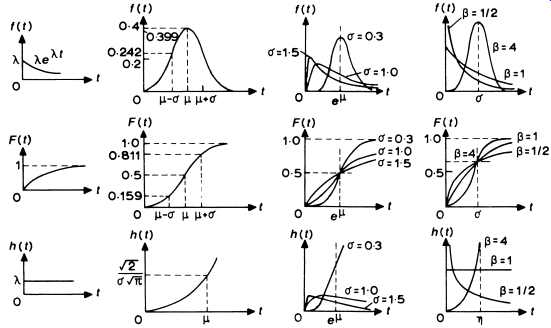
Fig. 5. Density, cumulative distribution, and hazard functions of
the exponential, normal, log-normal and Weibull distributions.
The reliability function. The function complementary to the cumulative distribution function is the reliability function, also called survival function. This function can be used to determine the probability that equipment will survive to a specified time t. The reliability function is denoted as R_t_ and is defined by:
R_t_ = _ t f_t_dt (4)
and, obviously:
R_t_ = 1-F_t_
The failure rate or hazard function. The last type of function derived from the other functions is the hazard function. It has other names in the literature, such as intensity function , force of mortality, and also failure rate in a certain context. It’s denoted as h_t_ and defined as:
h_t_ = f_t_ R_t_ = f_t_ 1-F_t_
The hazard function is a conditional probability that a system will fail during the time t and dt under the condition that the system is safe until time t. Someone once had a simple explanation of the hazard function.
It was made by analogy. Suppose someone takes an automobile trip of 200mil and completes the trip in 4 hr. The average travel rate was 50mph, although the person drove faster at some times and slower at others. The rate at any given instant could have been determined by reading the speed indicated on the speedometer at that instant. The 50mph is analogous to the failure rate and the speed of any point is analogous to the hazard rate.
The foregoing definitions rely on some rather involved mathematics.
The reader is referred to Green and Bourne and Henley and Kumamoto for more detailed explanations. However, we believe that there is no need to burden oneself with the mathematics of failure distributions. As we will see later, there has been considerable progress in the application of computerized models and appropriate software.
Specific distribution functions. A number of distributions have been proposed for machinery failure probabilities. Their definitions in terms of density function, cumulative distribution function, and hazard rate are depicted in Fig. 5.
The exponential distribution is the most important function due to its wide acceptance in the reliability analysis work of electronic systems. As shown in Fig. 5, this function is defined as:
f_t_ = _· exp_-_t_ for t _ 0
The exponential distribution is an appropriate model where failure of an item is due not to deterioration as a result of wear, but rather to random events. This feature of the exponential distribution also implies a constant hazard rate. The exponential distribution has been successfully applied as a time-to-failure model for complex systems consisting of a large number of components in series, none of which individually contributes significantly to the total failure density. This distribution is often used because of its universal applicability to systems that are repairable. Many kinds of electronic components follow an exponential distribution. Machinery parts behave in this mode when they succumb to brittle failure. For example, Fig. 6 shows that Diesel engine control unit failures followed an exponential distribution.
The normal distribution. Although the normal distribution has only limited applicability to life data, it’s used where failures are due to wear processes. The hazard or failure rate of this distribution cannot be expressed in a simple form.
The lognormal distribution is defined by:
f_t_ = 1 t_ v2_ exp
-_log_t/t50_ 2 2_2
where t50 = median = exp_u_, u = the mean of the logarithms of the times to failure,
_ = standard deviation.
The limited applicability of normal distribution to life data has been mentioned. This is not the case for the lognormal distribution which enjoys wide acceptance in reliability work. It has been applied in machinery maintainability consideration and where failure is due to crack propagation or corrosion. Nelson and Hayashi [8] give an exhaustive account of stress-temperature related furnace tube failure phenomena modeled by the lognormal distribution.
The Weibull distribution is defined by two parameters - , the nominal or characteristic life, * and a constant, a non-dimensional shape parameter. A typical Weibull distribution fit for life of a ball bearing is shown in Fig. 7.
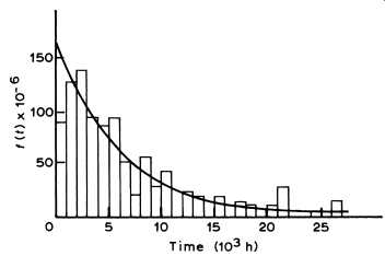
Fig. 6. Density function f_t_ of the failure of diesel engine control
units.
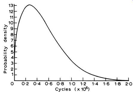
Fig. 7. Weibull function for a ball bearing. (Source: Sidall, J.N.,
Probabilistic Engineering Design, 1983, p. 361, Fig. 11-3, Marcel Dekker,
Inc.)
The ability of the Weibull function to model failure distributions makes it one of the most useful distributions for analyzing failure data.
If the shape parameter > 1, an increasing h_t_ is indicated which is symptomatic of wear-out failures. Where = 1, we find an exponential function, which obviously is a special case of the Weibull distribution.
With
= 1, a constant hazard or failure rate is indicated.
Where
= 2, this means that h_t_ is linearly increasing with t.
The resulting distribution is a special case of the Weibull function known as the Rayleigh distribution.
If
<1, a decreasing failure rate h_t_ is indicated. This would be typical for machinery components where run-in or initial self-accommodation takes place. Mechanical shaft seals would be a typical example.
The mean and standard deviation of the Weibull distribution involves complex calculations. For most engineering problems where the shape factor is greater than 0.5, they can be found from:
In cases where the shape factor is greater than 1, the mean is nearly equal to characteristic life _
_. The error involved in this assumption will generally be small compared to other errors stemming from the quality of data.
TBL. 1
Selected basic machinery component failure modes and their statistical distributions
Basic failure mode Exponential Normal Weibull
Probability distribution:
1.0 Force/stress
1.1 Deformation
1.2 Fracture
1.3 Yielding
2.0 Reactive environment
2.1 Corrosion
2.2 Rusting
2.3 Staining
3.0 Temperature/thermal
3.1 Creep
4.0 Time effects
4.1 Fatigue
4.2 Erosion
4.3 Wear
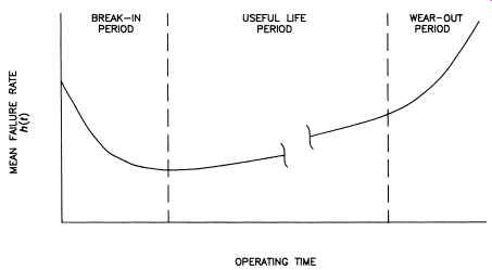
Fig. 8. Mean failure rate curve as a function of time.
One difficulty in attempting to fit theoretical distribution to failure or "life" data arises when a part or an assembly is subject to different failure modes. TBL. 1 lists some of the basic machinery component failure modes and shows the distributions they tend to follow. There are three different possibilities in which these failure modes appear:
1. Simultaneously with some time differences. Fit corrosion , for instance, in an anti-friction (ball) bearing would appear as wear first and then as corrosion. Sidall shows how to evaluate simultaneous failure mode occurrences in the context of failure distributions.
2. Failure modes occur singularly and exclusive of others. This is a somewhat theoretical assumption that we won’t deal with any further.
3. Amore realistic model can be created by assuming that failure modes occur consecutively in time. A commonly accepted concept is shown in Fig. 8. In this curve, called the bathtub curve, three conditions can be distinguished:
(1) early or infant mortality failures, (2) random failures, and (3) wear-out failures.
Condition 1 describes the early time period of a machinery system or part by showing a decreasing failure rate over time. It’s usually assumed that this period of "infant mortality" or "burn-in" is caused by the existence of material and manufacturing flaws together with assembly errors. Parts or systems that would exclusively exhibit this behavior would fit a Weibull distribution with
< 1. Condition 2, the area of constant failure rate, is the region of normal performance. This period is termed "useful life," during which time only random failures will occur. Parts or systems that would exclusively exhibit this failure behavior would fit a Weibull distribution with
= 1 or for that matter an exponential distribution. Condition 3 _
>1_ is characterized by an increase of failure
rate with time. As mentioned before, failures may be due to aging and wear out.
It has been said that the bathtub curve concept is purely theoretical and only serves the purpose of promoting a better understanding of failure events. However, real-world examples can be cited in connection with non-repairable parts. For example, if a large number of light bulbs or anti friction bearings operate continuously, some fail due to defects. During the useful life, occasional random failures occur, but most survive to old age, when the failure rate rises.
The bathtub curve pertaining to repairable components and their systems is rarely discussed in the reliability literature. However, most machinery components follow this curve. Its time axis is the cumulative operating time of the equipment, not the time interval between failures.
The major difference between this curve and the non-repairable curve is that it continues indefinitely or until the equipment is removed from service because it’s uneconomical to repair.
Estimation of Failure Distributions for Machinery Components
The data required to determine failure distributions are the individual times to failure of the equipment.
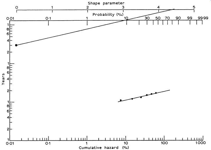
Fig. 9. Weibull hazard plot.
The procedure is to convert the data to become representative of the cumulative failure distribution F_t_. This is done by plotting times to failure against F_t_ on a scale which corresponds to the distribution to be fitted. For the exponential distribution this would be:
Consequently:
A plot of 1/_1-F_t_ on a log scale against time on a linear scale produces a straight line. For the Weibull distribution:
For most distributions, special graph papers are available which allow direct plotting of F_t_ versus t ( Fig. 9 illustrates a Weibull graph).
Nelson describes distributions and the fitting of life or failure data.
We encourage our readers to investigate the possible use of computer software packages developed for the statistical analysis of data relating to the failures and successful performance of machinery or components.
Their analysis capabilities range from simple calculations such as mean life, to the fitting of Weibull and other distribution models.
Application of Failure Distributions
The application of failure distributions for reliability predictions has been described in numerous references. With the emergence of improved data bases there is a new interest in these applications. Exhaustive information covering the application of distribution functions to equipment maintenance, replacement, and reliability decisions can be obtained , for example, from Jardine.
Our first example will cover a replacement decision in connection with large _>1500 hp_ electric motors in a petrochemical process plant. The motors considered for replacement had served this particular plant well for 18 years, but failure experience with similar motors at the same time had raised doubt in the owner's mind as to whether or not an 18-year-old motor could still be called reliable. All motors were 4000 kVA, 3 phase, 60 cycle, pipe-ventilated squirrel cage induction motors.
The failure experience of similar motors is listed in TBL. 2. Motors shown as having failed are denoted by a superscript _a _. These motors had stopped suddenly on-line through winding failures. Mean forced outage penalties were in the neighborhood of 1600 k$ considering the availability or unavailability of motor rewind shops and materials. The cost of an emergency rewind amounted to 125 k$, whereas the cost of a preventive rewind was 100 k$ with no penalty cost for loss of production. The problem was simply to balance the cost of preventive rewinds against their benefits. In order to do this one needs to determine the optimal preventive replacement age of the motor windings to minimize the total expected cost of replacement per unit time. Obviously, one requires a probabilistic model of the motor winding life in order to make a reliability assessment.
TBL. 2
Large motor winding failures: Failure data and hazard calculation
Motor Rank Years Hazard Cumulative hazard
Obtaining the Weibull Function
The Weibull function was obtained by plotting the data contained in TBL. 2 on appropriate Weibull paper ( Fig. 9).
The plotting method used has been proposed by Nelson for "multiply censored" life data consisting of times to failure on failed units, and running times - called censoring times - on unfailed units. The method is known as hazard plotting. It has been used effectively to analyze field and life test data on products consisting of electronic and mechanical parts ranging from small electric appliances to heavy industrial equipment. The hazard plotting method originally appeared in Nelson, which also contains more details.
Steps:
1. The n times, or years in our case, are placed in order from the smallest to the largest as shown in TBL. 2. The times are labeled with reverse ranks, that is the first time is labeled n, the second labeled n-1 , and the nth is labeled 1. The failure times are each marked by a superscript _a
_ to distinguish them from the censoring times.
2. Calculate a hazard value for each failure as 100/k, where k is its reverse rank. The hazard values for the large motor winding failures are shown in TBL. 2. For example, for the winding failure after 13 years, the reverse rank is 11 and the corresponding hazard value is 100/11 = 9_1%.
3. Proceed to calculate the cumulative hazard value for each failure as the sum of its hazard value and the cumulative hazard value of the preceding failure. For instance , for the motor failure after 13 years of operation, the cumulative hazard value of 25.12 is calculated by adding the hazard value of 9.1 to the cumulative hazard value of 16.03 of the preceding failure.
4. For plotting purposes, the hazard paper of a theoretical distribution of time to failure was chosen. The Weibull distribution seemed appropriate. On the vertical axis of the Weibull hazard paper, make a time-scale that includes the sample range of failure times (i.e., years).
5. Plot each failure time vertically against its corresponding cumulative value on the horizontal axis. The plot of the large motor winding failures is shown in Fig. 9. If the plot of the sample times to failure is reasonably straight on a hazard paper, one can conclude that the underlying distribution fits the data adequately. By eye, fit a straight line through the data points ( Fig. 9). Practical advice and more tips on making hazard plots are given by Nelson and King.
A hazard plot provides information on:
• the percentage of items failing by a given age;
• percentiles of the distribution;
• the behavior of the failure rate of the units as a function of their age;
• distribution parameters.
In our context we are mainly interested in the distribution parameters.
We already know that the Weibull distribution has an increasing or decreasing failure rate depending on whether its shape parameter has a value greater than, equal to, or less than 1. To obtain the shape parameter, draw a straight line parallel to the fitted line so it passes through the dot in the upper left-hand corner of the paper and through the shape parameter scale. Nautical chart parallel rulers are ideally suited for this task. Fig. 9 shows the result. The value on the shape parameter scale is the estimate and is ˆ - estimate of 4.3 suggests that the winding failure rate increases with age - that is, in a wear-out mode. It also suggests that the machines should be rewound at some age when they are too prone to failure.
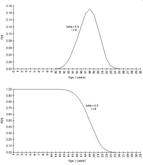
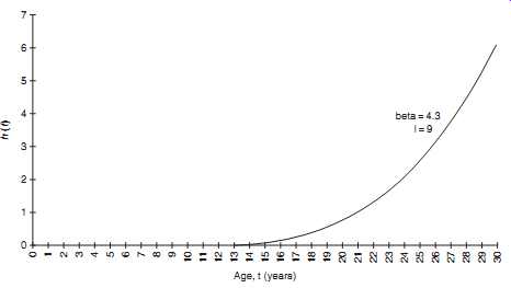
Fig. 10. (a) Probability density curve for large motor windings;
(b) reliability curve for large motor windings; (c) hazard curve for
large motor windings.
In order to estimate the other parameter of the Weibull function , we enter the hazard plot on the cumulative hazard scale at 100 or 63% on the probability scale. If we move up the fitting line on Fig. 9 and then sideways to the time-scale, we find the scale parameter, that is 18.5 years.
We now proceed to define the Weibull distribution function that describes the large motor winding population. We write:…
where t is the age of the motors ...is the characteristic life ... the shape parameter l is the location parameter The location parameter, l, takes into account that our motors did not begin to fail before age 9-10. On the other hand, l would be equal to zero when it’s expected that failures appear as soon as an item is placed into service and:
Applying the estimated parameters ˆ and ˆ , Fig. 10 was produced by using a simple computer program. After having made this reliability assessment one can now proceed to work the economic decision of how to optimize motor replacement.
Construction of the Replacement Model
The construction of the replacement model is credited to A. K. S. Jardine and A. D. S. Carter.
1. Cp is the cost of preventive replacement.
2. Cf is the cost of forced outage replacement.
3. f_t_ is the probability density function of the failure times of the motor windings.
4. The replacement strategy is to preventively replace the motors or their windings once they have reached a specified age tp. Also, there will be replacement upon failures as necessary. This strategy is shown in Fig. 11.
5. The goal is to determine the optimal replacement age of the motor windings to minimize the total expected replacement cost per unit time.
The equation describing the model of relating replacement age tp to total expected replacement cost per unit time is:
For the motor winding replacement case:
The numerical solution to the problem is presented in TBL. 3.
The various columns of TBL. 3 show the values of the variables in equation 4.17 as a function of tp. Finally, Fig. 12 illustrates C_tp_ and shows that the optimal decision would have been to preventively rewind the company's large motors after 11-12 years.
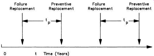
Fig. 11. Large motor replacement strategy.
TBL. 3 Calculation results for large motor replacement case
The petrochemical company obviously missed out on optimizing its large motor rewind strategy, given the validity of the Weibull function based model. The question arose whether or not it would now be economical, into the 19th year of their large motor operations, to plan for a preventive rewind of their three oldest motors during an upcoming shut down. Using the relationship: Incentives or cost of insurance =Cf ×h_tp_ annual penalties for the next five years* were determined as shown in column 7 of TBL. 3. These amounts were in turn claimed as credits in a discounted cash flow (DCF) analysis. They felt it was a sound decision to preventively rewind their three old motors during the shutdown.
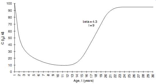
Fig. 12. Expected replacement cost as a function of time.
Our second example involves the analysis of predominant failure regimes of process plant machinery.
Here our goal was to arrive at appropriate intervals for rebuilding pumps and motors in a major petrochemical plant.
The maintenance philosophy in this plant required that pumps and motors be rebuilt on a periodic basis of either the running hours or time in service. The rebuild criterion was water pumps to be rebuilt after 8000 hr, crude oil pumps after 16,000 hr, and motors after 20,000 hr. A unit was also rebuilt after five years if it had not reached its run-time limit. The primary assumption behind a criterion such as this is that machines deteriorate or wear out with time or during operation and should be removed from service prior to failure.
In order to evaluate the rebuild criteria just mentioned, the bathtub curve must be determined that characterizes the life of pumps and motors by establishing the relationship of failure rate with time.
Here, Hazard Analysis is used to analyze the run-time data to establish the predominant failure distribution and the median life of the units. The time to failure for each incident is plotted against the summation of the hazard function. This is shown in Fig. 13. When the data are plotted on log-log format, the results are somewhat similar to that of the bathtub curve.
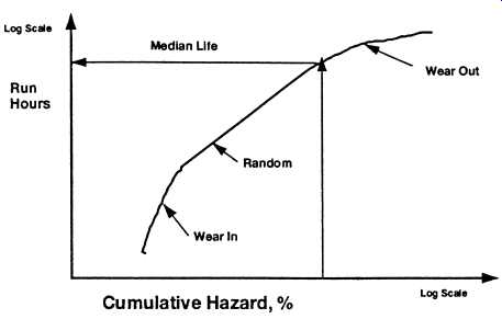
Fig. 13. Hazard analysis plot.
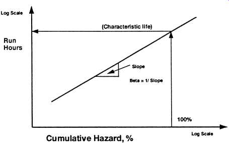
Fig. 14. Hazard analysis plot showing the Weibull parameters, h and
b.
If proper Weibull hazard plotting paper, as shown in Fig. 9, is not available, can be determined as the reciprocal of the slope of the plotted data as demonstrated in Fig. 14. Consequently , for a hazard that decreases with time, a "wear-in" failure rate, the data will plot on a curve that has a slope greater than unity _ < 1_. For failures that follow a constant failure rate distribution, the data points will fall on a curve that has a slope of unity _ = 1_, and for "wear-out" distributions, the slope is less than unity _ > 1_.
For large populations, all three distributions may be present and the data will resemble a bathtub that is inverted and rotated upward by 45 degr.
However, when the data plot as a straight line on log-log coordinates, a Weibull distribution can be fitted to the data.
Because the failures of the pumps and motors in this study generally have several different failure modes, the data may not fall on a straight line that can be fitted to a single Weibull distribution. For those cases, the life of the population will be taken as the median life ___, or that time when 50% of the units have failed. On a hazard plot, the median life is determined where the fitted curve crosses the "Cumulative Hazard" value of 100%, which is equivalent to a 63.2% failure probability.
As in our previous example, we have to analyze data that are multiply censored, that is, failure data that are incomplete. Our group of machines being analyzed may have many machines that have not yet failed. They either may still be in operation or may have been removed from service for reasons other than failure. The machines that were removed for rebuild are in this category. This group of machinery has accumulated significant running hours, and although these machines have not failed, their running time must be factored into any life estimate.
Data Sources
Several sources of data were used to determine the life of pumps and motors. The most useful information is contained in the "Run-time Report," a report that is generated from a computer data base that contains the current running hours of the equipment that was installed previously in a given location. From this information a hazard analysis can be made.
However, the use of the Run-time Report by itself as a source of failure data has a significant weakness in that it does not record whether a machine was removed because it failed or because it was taken out to be rebuilt or for some other reason.
To determine if a machine was removed from service because of failure or because it had met one of the rebuild criteria, a report was available in which the rebuilds were scheduled for work based upon their running or installed hours. It’s general practice to schedule a rebuild when a machine reaches 80% of the run-time criteria or when it would exceed the 5-year criteria in the next year. This report is issued yearly and lists those machines that are scheduled for rebuild in the coming year. By cross referencing information in both the Run-time Report and the Rebuild Schedule, it was generally possible to determine whether a machine was removed because it met a rebuild criterion or whether it failed. If a unit could not be found on the Rebuild Schedule and conversations with field personnel could not rule out a failure, the machine was considered to have failed in service. Because of the state of the data, a degree of judgment was sometimes required in making this assessment. As long as the number of data points is large, a few errors in the data should not significantly influence the overall conclusions drawn from the analysis. This would not be true if a small number of machines or data points was considered.
The Rebuild History Report summarizes the run-time of a given unit every time it’s rebuilt. The data from this report were used to deter mine the effect that rebuilding had on machine life. Although the report included information for both pumps and motors, only motors were considered in this analysis. Pumps were excluded from this analysis because the data included a mix of carbon steel and stainless steel (SS) pumps.
A material change for some pumps occurred during the time period of the data. It was felt that the improvement in pump life due to the introduction of SS pumps precluded a meaningful comparison of the units based on the number of rebuilds.
For the purpose of determining the failure rate and life of the equipment, the Rebuild History Report suffers from the same problems as the Run-time Report. The data don’t indicate if the motor had failed prior to removal from service. The run-time data from the report were cross-referenced with those of the Rebuild Schedule to arrive at a judgment as to whether or not a machine had failed. Because of the large number of data points, some errors in discriminating between failures and non-failures should not affect the overall conclusions. However , for machines with over five rebuilds, there are too few data points for valid conclusions to be drawn.
The documentation of rebuild information in the Rebuild History Report did not include rebuild information prior to the date that the report was issued. Much of the equipment had been reworked several times before that date; thus, any analysis concerning the cumulative hours and rebuilds on the motors would be incomplete. The analysis cannot therefore determine the life of the original motors and is thus restricted to effect of rebuilds on machinery life after several unknown number of rebuilds. This limitation is of a particular concern when the existing motor life is compared with industry experience.
Analysis of Run-Time Data
To assist in manipulating the data for a Hazard Analysis, several Relational Data Bases (RDB) were constructed that contained machinery information to correlate pump and motor reliability. For both pumps and motors, a RDB was constructed that included such factors as location, machine type, service, speed, and performance. A separate "Run-time" RDB was produced that included such data as location, run-time, and failure mode. These two were linked through the location parameter to produce a file that was compatible with a Hazard Analysis Program. A third "Rebuild" RDB for motors that deals with the number of documented rebuilds was also produced. This process is illustrated in Fig. 15.
To perform an analysis, the database with the particular characteristics of interest and the data base with the failure information are linked through the equipment location number to extract the running hours and failure mode. This data is exported as a file to the Hazard Analysis Program that produces the plot. This method allows for the investigation of a wide variety of questions on equipment reliability and is limited only by the amount of data. For example, the analysis can determine the life and predominant failure mode of all crude oil pumps at a particular site.
Another very powerful use of this analysis is the capability of determining the results of design modifications.
===
Motor Information Speed, HP, etc.
Motor Run Time Data Hazard (Weibull) Analysis Motor Rebuild History
Pump Run Time Data
Pump Information Speed, HP, Flow, etc.
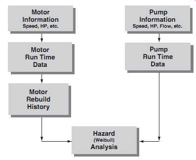
Fig. 15. Analysis process linking relational data bases with hazard
analysis.
===
Analysis of Pumps
To evaluate the rebuild criteria for pumps, the Pump RDB and the Pump Run-time RDB were linked and the data extracted using a select criterion of pump service. Pumps in water and crude oil services were selected for this study.
The Hazard Analysis Plot for the water pumps is given in Fig. 16.
This figure indicates that the water pumps have a median life of approximately 9000 hr compared to the rebuild criteria of 8000 hr. Half of the water pumps fail before 9000 hr and half after that time.
For the first portion of the curve in Fig. 16, the slope of the data is approximately 2.7 _ = 0_36_, indicating a "wear-in" type of failure mode. At about 1800 running hours, the failure mode changes to a constant failure rate mode. At no time do the data indicate that the pumps are failing in a predominantly "wear-out" mode.
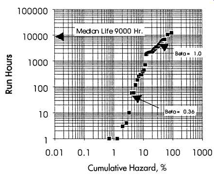
Fig. 16. Hazard analysis of water pumps.
The significant number of machines that fail before 1800 hr indicates that either the pumps are not being rebuilt properly or that they are being installed incorrectly. However, the lack of documentation of failures precludes an analysis that might determine the reasons for such early failure. Although a statistical analysis such as this cannot offer detailed explanations of the cause of failures, it can determine general failure modes. The number of machines that are shown to suffer from a wear in failure mode raises a strong concern about the operating and cost effectiveness of the current rebuild philosophy. Removing a machine from its location, disassembling, reassembling, storing, and reinstalling exposes a machine to significant risk of damage and mishap.
At about 1800 hr, the figure shows a significant change in the slope of the data. The slope becomes unity _ = 1_0_, which indicates the failures become random with time. That is, the chance of a failure becomes independent of the time that the machine went into service. An example of this mechanism would be the accidental closing of a discharge valve that caused a pump to run dead-headed and fail. The timing of the valve closing would not, in general, be a function of when the unit went into service, and thus the failure is random. Many operational and environmental causes of failure fall into this category.
The analysis of crude oil pumps shows a somewhat similar pattern to that of the water pumps. The hazard plot for these data is shown in Fig. 17. The plot indicates that the median life of these units is only about 6600 hr. There is no indication in the data that the crude oil pumps have significant wear-out modes. This is not to say that a few individual pumps might not wear-out, only that the bulk of the population suffers from a wear-in or random failure. The longer the pumps are left in service, the lower the overall failure rate becomes. The plot of failure data in Fig. 17 has a slope of approximately 2.0 _ = 0_5_ indicating a wear-in mode over most of the life of the machines.
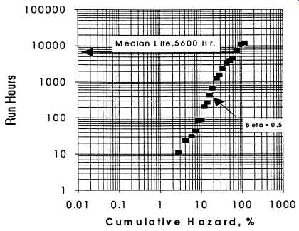
Fig. 17. Hazard analysis of crude oil pumps.
Analysis of Motors
The run-time data were analyzed for all critical motors. The hazard analysis plot is shown in Fig. 18. This plot indicates that the median life of the motors is approximately 13,000 hr. Up until that time, the failures are predominantly a "wear-in" or "infant mortality" mode. At about 13,000 hr, the plotted data change to a that is greater than one, indicating that the motors begin to wear out. This is seen in Fig. 18, where the data shifts from a slope of approximately 1.7 _ = 0_57_ to a slope of about 0.6 _=1_7_. Of all of the cases that were analyzed, motors seem to be the only ones that reach a significant wear-out mode that might justify a rebuild philosophy based upon running hours. However, even this conclusion may not be valid because rebuilding the motors, like the pumps, introduces significant "infant mortality" failures.
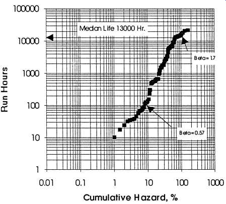 Fig. 18. Hazard analysis of motors.
Analysis of Rebuild Data
In addition to the run-time data that were analyzed above, there also exists information that relates the life of pumps and motors as a function of the number of times that they are rebuilt. Here, only the motors will be studied. The pump rebuild information has run-time data that includes a mix of carbon steel and stainless steel cases. The introduction of SS pumps, while significantly improving the life of the units, complicates the analysis when attempting to study the effects of pump rebuild. The rebuild data consists of a group of carbon steel pumps that includes an unknown number of rebuilds and cumulative running hours and SS pumps that are newer. Attempting to separate all of these variables to determine the effect of rebuilds on pumps was judged to be unproductive.
Had the failure and run-time data been available at the beginning of the plants and been more complete, the hazard analysis tools would have been invaluable in quantifying the improvements in reliability of the pumps due to the material change.
The rebuild data for the motors were analyzed in a similar manner to that described above for the run-time data. To study the effect that rebuilding has on a machine's life, the data were organized by the number of times the motor had been rebuilt. The data are only valid since 1981; therefore, the first "documented" rebuild probably does not rep resent the first "actual" rebuild. For the purposes of this study, the first "documented" rebuild will be referred to simply as the "first" rebuild.
As was the case with the run-time data, the information on the rebuild does not indicate that a machine was removed because of failure. Using the same criteria as described above, it was assumed that a machine had not failed if it were near its rebuild run-time or five-year criteria or if it was on the Rebuild Schedule. Otherwise, it was assumed that a machine had failed for some reason. It’s recognized that this assumption will introduce some error in the analysis; however, it’s felt that this would not significantly change the conclusions as long as the population under consideration was reasonably large.
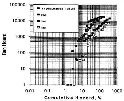
Fig. 19. Hazard plots of rebuilt motors.
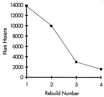 Fig. 20. Median motor life as a function of number of rebuilds.
Fig. 19 presents the Hazard Analysis of the rebuild data for the first four documented rebuilds of the motors. There were up to seven rebuilds for some motors, but it was felt that the sample population was not large enough to use without introducing significant errors. As seen in the plots, the median life decreases with the number of rebuilds. This is seen more clearly when the median life of each rebuild is plotted in Fig. 20.
In this figure, the motor life for the first rebuild is approximately 14,000 hr and decreases to about 1600 hr for the fourth rebuild. This data indicates that every time the motors are rebuilt or reconditioned, the life decreases and motors are not brought back to "like new" condition.
Fig. 20 indicates that many of the motors may have reached the end of their economic life and should be replaced. A motor rebuild cost can be substantial, and the data shows that after about three rebuilds, this expenditure extends the life of the machine only a few months of run-time.
Examination of the individual curves in Fig. 19 indicates that only the motors represented by the first rebuild have a significant wear-out mode and that all of the motors are subjected to infant mortality failures. For the first rebuild case, the failures shift from a wear-in to a wear-out mode that occurs at approximately 9000 hr. After this first documented rebuild, the failures are "wear-in" changing to "random." As was concluded for the current motor population discussed earlier, a large percentage of machines suffer from early failures after they are reinstalled.
Because the failure documentation system was incomplete, the reasons or causes for these failures could not be determined. However, common causes of a high infant mortality in machines are generally recognized as due to poor or marginal design, poor assembly, or bad installation. For any of these conditions, a machine can fail soon after installation.
The current state of the failure history documentation does not permit a determination of the exact causes for the decrease in life of the motors because they are repeatedly rebuilt. However, some general conclusions can be made. For pumps, a rebuild that replaces all of the internal components can restore it to a "like new" condition, at least in theory. This is not the case for a motor. The normal reconditioning of a motor does not replace the stator windings and insulation, which will continue to degrade with time. Thus, the insulation on a motor that has been rebuilt several times may be over 15-20 years old and approaching the end of its useful life. When the motor is rewound, it still is not totally restored.
To remove the old winding and insulation, the stator is heated in an oven to burn out the insulation. Although care is taken to avoid any damage to the rest of the stator, some deterioration is unavoidable in the thin varnish insulation between the stator iron laminations. When this insulation is damaged, eddy current losses increase and the motor will run hotter than before the rewind.
Another element of motors that is not corrected by a rebuild is rotor bar thermal fatigue. Each motor start will subject the rotor bars to high temperature and cyclic stresses. Eventually this can cause rotor bar cracking and failure.
The fact that motors are never fully reconditioned is probably reflected in the decrease in life shown in Fig. 20. However, because the rebuild data does not include the early portion of a motor's life, it was not always possible to separate the effects of age from the number of rebuilds.
The availability estimates currently used to establish sparing levels was based upon the assumption of a constant failure rate. However, the rebuild philosophy had the effect of resetting the clock on the machines and keeping them in a wear-in mode where the actual failure rate is higher than that assumed. Because the failure rate is shown to be a function of time, an accurate assessment of the impact on machinery availability must consider the installed time for individual machines except in the random regime.
Life Comparison With Other Industrial Experience:
The current life of the motors in the study does not compare favorably with the experience of industry. Two industrial surveys of motor life and the factors that influence life are presented in Institute of Electrical and Electronic Engineers (IEEE) studies and Electrical Power Research Institute (EPRI) studies. The IEEE study includes reliability data for a population of 1141 motors, 200 horsepower (hp) and above. This study covers a wide range of different types of industrial users. The EPRI study addresses only the utility industry, but covers a large population of 6312 motors. The EPRI study considers only motors of 200 hp and above. Of the two, the IEEE study, with its greater diversity of industrial applications and exposed equipment, is probably more representative of the type of service and environment that is found in the facilities of this study.
A comparison of the average life of motors in industry as compared to motor life in the study is shown in Fig. 21. In this figure, the life of motors in the IEEE study is 14 years, and the life in the EPRI study is 31 years. This compares with the life of the study motors of 1.4 years, and for motors that have been rebuilt at least 4 times of 0.18 years. It should be noted that the IEEE and the EPRI studies deal with average or mean life, and this data is for median life. For wear-out types of failures, the mean and the median are the same. However , for populations such as those of this study, where the predominant failures are wear-in or random modes, the median life is less than the mean or average.
=========
0 LIFE YEAR'S MOTOR LIFE INDUSTRY IEEE INDUSTRY EPRI STUDY MOTORS REBUILDS
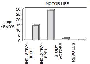
Fig. 21. Comparison of life of study motors with industrial experience.
=========
Conclusion
The statistical analysis used in this study indicated that the rebuild philosophy used to maintain the population of pumps was detrimental to the reliability of the units. Removing the machines from service based upon an arbitrary schedule of running time or time in service introduced failure modes that resulted in an increase in infant mortality. It was recommended to the client that a predictive maintenance program be implemented in the plants so that maintenance would be performed based upon the measured condition of the machinery. Also, early detection of faults with a monitoring program would allow for repairs to be performed in situ at much less expense than totally rebuilding a unit at an outside facility.
The failure analysis and maintenance documentation system for the facilities did not permit a detailed analysis of the failure modes of the equipment. It was recommended to the client that this system be upgraded so that the specific problem areas could be addressed in the future.
(also see Process Plant Machinery: Electric Motors and Controls)
Prev. | Next