AMAZON multi-meters discounts AMAZON oscilloscope discounts
AMAZON multi-meters discounts
AMAZON oscilloscope discounts
.
.All mechanical equipment in motion generates a vibration profile, or signature,
that reflects its operating condition. This is true regardless of speed or
whether the mode of operation is rotation, reciprocation, or linear motion.
Vibration analysis is applicable to all mechanical equipment, although a common-yet
invalid-assumption is that it’s limited to simple rotating machinery with running
speeds above 600 revolutions per minute (rpm). Vibration-profile analysis is
a useful tool for predictive maintenance, diagnostics, and many other uses.
Predictive maintenance has become synonymous with monitoring vibration characteristics of rotating machinery to detect budding problems and to head off catastrophic failure; however, vibration analysis does not provide the data required for analyzing electrical equipment, areas of heat loss, the condition of lubricating oil, or other parameters typically evaluated in a maintenance management program. Therefore, a total plant predictive maintenance program must include several techniques, each designed to provide specific information on plant equipment.
VIBRATION ANALYSIS APPLICATIONS
The use of vibration analysis is not restricted to predictive maintenance. This technique is useful for diagnostic applications as well. Vibration monitoring and analysis are the primary diagnostic tools for most mechanical systems that are used to manufacture products. When used properly, vibration data provide the means to maintain optimum operating conditions and efficiency of critical plant systems. Vibration analysis can be used to evaluate fluid flow through pipes or vessels, to detect leaks, and to perform a variety of nondestructive testing functions that improve the reliability and performance of critical plant systems.
==========
TBL. 1 Equipment and Processes Typically Monitored by Vibration Analysis
Centrifugal Reciprocating Continuous Process Pumps; Pumps Continuous Casters Compressors; Compressors Hot and Cold Strip Lines Blowers Diesel Engines Annealing Lines Fans Gasoline Engines Plating Lines Motor/Generators Cylinders Paper Machines Ball Mills Other Machines Can Manufacturing Lines Chillers Pickle Lines Product Rolls Machine-Trains Printing Mixers Boring Machines Dyeing and Finishing Gearboxes; Hobbing Machines Roofing Manufacturing Lines Centrifuges Machining Centers Chemical Production Lines Transmissions Temper Mills Petroleum Production Lines Turbines Metal Working Machines Neoprene Production Lines Generators Rolling Mills, and Most Polyester Production Lines Rotary Dryers Machining Equipment Nylon Production Lines Electric Motors Flooring Production Lines All Rotating Machinery Continuous Process Lines
===========
Some of the applications that are discussed briefly in this section are predictive maintenance, acceptance testing, quality control, loose part detection, noise control, leak detection, aircraft engine analyzers, and machine design and engineering. TBL. 1 lists rotating, or centrifugal, and nonrotating equipment, machine-trains, and continuous processes typically monitored by vibration analysis.
Predictive Maintenance
The fact that vibration profiles can be obtained for all machinery having rotating or moving elements allows vibration-based analysis techniques to be used for predictive maintenance. Vibration analysis is one of several predictive maintenance techniques used to monitor and analyze critical machines, equipment, and systems in a typical plant. As indicated before, however, the use of vibration analysis to monitor rotating machinery to detect budding problems and to head off catastrophic failure is the dominant technique used with maintenance management programs.
Acceptance Testing
Vibration analysis is a proven means of verifying the actual performance versus design parameters of new mechanical, process, and manufacturing equipment. Pre-acceptance tests performed at the factory and immediately after installation can be used to ensure that new equipment performs at optimum efficiency and expected life-cycle cost.
Design problems as well as possible damage during shipment or installation can be corrected before long-term damage and/or unexpected costs occur.
Quality Control
Production-line vibration checks are an effective method of ensuring product quality where machine tools are involved. Such checks can provide advanced warning that the surface finish on parts is nearing the rejection level. On continuous-process lines such as paper machines, steel-finishing lines, or rolling mills, vibration analysis can prevent abnormal oscillation of components that result in loss of product quality.
Loose or Foreign Parts Detection
Vibration analysis is useful as a diagnostic tool for locating loose or foreign objects in process lines or vessels. This technique has been used with great success by the nuclear power industry, and it offers the same benefits to nonnuclear industries.
Noise Control
Federal, state, and local regulations require that serious attention be paid to noise levels within the plant. Vibration analysis can be used to isolate the source of noise generated by plant equipment as well as background noises such as those generated by fluorescent lights and other less obvious sources. The ability to isolate the source of abnormal noises permits cost-effective corrective action.
Leak Detections
Leaks in process vessels and devices such as valves are a serious problem in many industries. A variation of vibration monitoring and analysis can be used to detect leakage and isolate its source. Leak-detection systems use an accelerometer attached to the exterior of a process pipe. This allows the vibration profile to be monitored in order to detect the unique frequencies generated by flow or leakage.
Aircraft Engine Analyzers
Adaptations of vibration-analysis techniques have been used for a variety of specialty instruments, in particular portable and continuous aircraft engine analyzers. Vibration monitoring and analysis techniques are the basis of these analyzers, which are used to detect excessive vibration in turbo-prop and jet engines. These instruments incorporate logic modules that use existing vibration data to evaluate the engine condition.
Portable units have diagnostic capabilities that allow a mechanic to determine the source of the problem while continuous sensors alert the pilot of any deviation from optimum operating condition.
Machine Design and Engineering
Vibration data have become a critical part of the design and engineering of new machines and process systems. Data derived from similar or existing machinery can be extrapolated to form the basis of a preliminary design. Prototype testing of new machinery and systems allows these preliminary designs to be finalized, and the vibration data from the testing add to the design database.
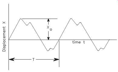
FIG. 1 Periodic motion for bearing pedestal of a steam turbine.
VIBRATION ANALYSIS OVERVIEW
Vibration theory and vibration profile, or signature, analyses are complex subjects that are the topic of many textbooks. This section provides enough theory to allow the concept of vibration profiles and their analysis to be understood before beginning the more in-depth discussions in the later sections of this book.
Theoretical Vibration Profiles
A vibration is a periodic motion or one that repeats itself after a certain interval. This interval is referred to as the period of the vibration, T. A plot, or profile, of a vibration is shown in FIG. 1, which shows the period, T, and the maximum displacement or amplitude, X0. The inverse of the period, __ , is called the frequency, f, of the vibration, which can be expressed in units of cycles per second (cps) or Hertz (Hz).
A harmonic function is the simplest type of periodic motion and is shown in FIG. 2, which is the harmonic function for the small oscillations of a simple pendulum.
Such a relationship can be expressed by the equation:
where:
X = Vibration displacement (thousandths of an inch, or mils) X0 = Maximum displacement or amplitude (mils) w = Circular frequency (radians per second) t = Time (seconds) XX t = () 0 sin w 1 T
Actual Vibration Profiles
The process of vibration analysis requires gathering complex machine data and deciphering it. As opposed to the simple theoretical vibration curves shown in FIGS. 1 and 2, the profile for a piece of equipment is extremely complex because there are usually many sources of vibration. Each source generates its own curve, but these are essentially added together and displayed as a composite profile. These profiles can be displayed in two formats: time-domain and frequency-domain.
Time-Domain:
Vibration data plotted as amplitude versus time is referred to as a time-domain data profile. Some simple examples are shown in FIGS. 1 and 2. An example of the complexity of this type of data for an actual piece of industrial machinery is shown in FIG. 3.
Time-domain plots must be used for all linear and reciprocating motion machinery.
They are useful in the overall analysis of machine-trains to study changes in operating conditions; however, time-domain data are difficult to use. Because all the vibration data in this type of plot are added together to represent the total displacement at any given time, it’s difficult to directly see the contribution of any particular vibration source.
The French physicist and mathematician Jean Fourier determined that non-harmonic data functions such as the time-domain vibration profile are the mathematical sum of simple harmonic functions. The dashed-line curves in FIG. 4 represent discrete harmonic components of the total, or summed, non-harmonic curve represented by the solid line.
This type of data, which is routinely taken over the life of a machine, is directly com parable to historical data taken at exactly the same running speed and load; however, this is not practical because of variations in day-to-day plant operations and changes in running speed. This significantly affects the profile and makes it impossible to compare historical data.
FIG. 3 Example of a typical time-domain vibration profile for a piece of machinery.
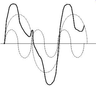
FIG 4 Discrete (harmonic) and total (non-harmonic) time-domain vibration
curves.
FIG. 5 Typical frequency-domain vibration signature.
Frequency-Domain
From a practical standpoint, simple harmonic vibration functions are related to the circular frequencies of the rotating or moving components. Therefore, these frequencies are some multiple of the basic running speed of the machine-train, which is expressed in revolutions per minute (rpm) or cycles per minute (cpm). Determining these frequencies is the first basic step in analyzing the operating condition of the machine-train.
Frequency-domain data are obtained by converting time-domain data using a mathematical technique referred to as Fast Fourier Transform (FFT). FFT allows each vibration component of a complex machine-train spectrum to be shown as a discrete frequency peak. The frequency-domain amplitude can be the displacement per unit time related to a particular frequency, which is plotted as the Y-axis against frequency as the X-axis. This is opposed to time-domain spectrums that sum the velocities of all frequencies and plot the sum as the Y-axis against time as the X-axis. An example of a frequency-domain plot or vibration signature is shown in FIG. 5.
Frequency-domain data are required for equipment operating at more than one running speed and all rotating applications. Because the X-axis of the spectrum is frequency normalized to the running speed, a change in running speed won’t affect the plot.
A vibration component that is present at one running speed will still be found in the same location on the plot for another running speed after the normalization, although the amplitude may be different.
Interpretation of Vibration Data
The key to using vibration signature analysis for predictive maintenance, diagnostic, and other applications is the ability to differentiate between normal and abnormal vibration profiles. Many vibrations are normal for a piece of rotating or moving machinery. Examples of these are normal rotations of shafts and other rotors, contact with bearings, gear-mesh, and so on. Specific problems with machinery generate abnormal, yet identifiable, vibrations. Examples of these are loose bolts, misaligned shafts, worn bearings, leaks, and incipient metal fatigue.
Predictive maintenance using vibration signature analysis is based on the following facts, which form the basis of the methods used to identify and quantify the root causes of failure:
• All common machinery problems and failure modes have distinct vibration frequency components that can be isolated and identified.
• A frequency-domain vibration signature is generally used for analysis because it consists of discrete peaks, each representing a specific vibration source.
• There is a cause, referred to as a forcing function, for every frequency component in a machine-train's vibration signature.
• When the signature of a machine is compared over time, it will repeat until some event changes the vibration pattern (i.e., the amplitude of each distinct vibration component will remain constant until the operating dynamics of the machine-train change).
Although an increase or decrease in amplitude may indicate degradation of the machine-train, this is not always the case. Variations in load, operating practices, and a variety of other normal changes also change the amplitude of one or more frequency components within the vibration signature. In addition, it’s important to note that a lower amplitude does not necessarily indicate an improvement in the mechanical condition of the machine-train. Therefore, it’s important that the source of all amplitude variations be clearly understood.
Vibration-Measuring Equipment
Vibration data are obtained by the following procedure: (1) mounting a transducer onto the machinery at various locations, typically machine housing and bearing caps, and (2) using a portable data-gathering device, referred to as a vibration monitor or analyzer, to connect to the transducer to obtain vibration readings.
Transducers:
The transducer most commonly used to obtain vibration measurements is an accelerometer. It incorporates piezoelectric (i.e., pressure-sensitive) films to convert mechanical energy into electrical signals. The device generally incorporates a weight suspended between two piezoelectric films. The weight moves in response to vibration and squeezes the piezoelectric films, which sends an electrical signal each time the weight squeezes it.
Portable Vibration Analyzers:
The portable vibration analyzer incorporates a microprocessor that allows it to mathematically convert the electrical signal to acceleration per unit time, perform an FFT, and store the data. It can be programmed to generate alarms and displays of the data.
The data stored by the analyzer can be downloaded to a PC or a more powerful computer to perform more sophisticated analyses, data storage and retrieval, and report generation.
VIBRATION SOURCES
All machinery with moving parts generates mechanical forces during normal operation. As the mechanical condition of the machine changes because of wear, changes in the operating environment, load variations, and so on, so do these forces. Under standing machinery dynamics and how forces create unique vibration frequency components is the key to understanding vibration sources.
Vibration does not just happen. There is a physical cause, referred to as a forcing function, and each component of a vibration signature has its own forcing function. The components that make up a signature are reflected as discrete peaks in the FFT or frequency-domain plot.
The vibration profile that results from motion is the result of a force imbalance. By definition, balance occurs in moving systems when all forces generated by, and acting on, the machine are in a state of equilibrium. In real-world applications, however, there is always some level of imbalance, and all machines vibrate to some extent. This section discusses the more common sources of vibration for rotating machinery, as well as for machinery undergoing reciprocating and/or linear motion.
Rotating Machinery
A rotating machine has one or more machine elements that turn with a shaft, such as rolling-element bearings, impellers, and other rotors. In a perfectly balanced machine, all rotors turn true on their centerline and all forces are equal. In industrial machinery, however, it’s common for an imbalance of these forces to occur. In addition to imbalance generated by a rotating element, vibration may be caused by instability in the media flowing through the rotating machine.
Rotor Imbalance:
Mechanical imbalance is not the only form of imbalance that affects rotating elements.
It’s the condition where more weight is on one side of a centerline of a rotor than on the other. In many cases, rotor imbalance is the result of an imbalance between centripetal forces generated by the rotation. The source of rotor vibration can also be an imbalance between the lift generated by the rotor and gravity.
Machines with rotating elements are designed to generate vertical lift of the rotating element when operating within normal parameters. This vertical lift must overcome gravity to properly center the rotating element in its bearing-support structure; however, because gravity and atmospheric pressure vary with altitude and barometric pressure, actual lift may not compensate for the downward forces of gravity in certain environments. When the deviation of actual lift from designed lift is significant, a rotor may not rotate on its true centerline. This offset rotation creates an imbalance and a measurable level of vibration.
Flow Instability and Operating Conditions:
Rotating machines subject to imbalance caused by turbulent or unbalanced media flow include pumps, fans, and compressors. A good machine design for these units incorporates the dynamic forces of the gas or liquid in stabilizing the rotating element. The combination of these forces and the stiffness of the rotor-support system (i.e., bearing and bearing pedestals) determine the vibration level. Rotor-support stiffness is important because unbalanced forces resulting from flow instability can deflect rotating elements from their true centerline, and the stiffness resists the deflection.
Deviations from a machine's designed operating envelope can affect flow stability, which directly affects the vibration profile. For example, the vibration level of a centrifugal compressor is typically low when operating at 100 percent load with laminar airflow through the compressor; however, a radical change in vibration level can result from decreased load. Vibration resulting from operation at 50 percent load may increase by as much as 400 percent with no change in the mechanical condition of the compressor. In addition, a radical change in vibration level can result from turbulent flow caused by restrictions in either the inlet or discharge piping.
Turbulent or unbalanced media flow (i.e., aerodynamic or hydraulic instability) does not have the same quadratic impact on the vibration profile as that of load change, but it increases the overall vibration energy. This generates a unique profile that can be used to quantify the level of instability present in the machine. The profile generated by unbalanced flow is visible at the vane- or blade-pass frequency of the rotating element. In addition, the profile shows a marked increase in the random noise generated by the flow of gas or liquid through the machine.
Mechanical Motion and Forces:
A clear understanding of the mechanical movement of machines and their components is an essential part of vibration analysis. This understanding, coupled with the forces applied by the process, is the foundation for diagnostic accuracy.
Almost every unique frequency contained in the vibration signature of a machine-train can be directly attributed to a corresponding mechanical motion within the machine.
For example, the constant endplay or axial movement of the rotating element in a motor-generator set generates elevated amplitude at the fundamental (1X), second harmonic (2X), and third harmonic (3X) of the shaft's true running speed. In addition, this movement increases the axial amplitude of the fundamental (1X) frequency.
Forces resulting from air or liquid movement through a machine also generate unique frequency components within the machine's signature. In relatively stable or laminar-flow applications, the movement of product through the machine slightly increases the amplitude at the vane- or blade-pass frequency. In more severe, turbulent-flow applications, the flow of product generates a broadband, white-noise profile that can be directly attributed to the movement of product through the machine.
Other forces, such as the side load created by V-belt drives, also generate unique frequencies or modify existing component frequencies. For example, excessive belt tension increases the side load on the machine-train's shafts. This increase in side load changes the load zone in the machine's bearings. The result of this change is a marked increase in the amplitude at the outer-race rotational frequency of the bearings.
Applied force or induced loads can also displace the shafts in a machine-train. As a result the machine's shaft will rotate off-center, which dramatically increases the amplitude at the fundamental (1X) frequency of the machine.
Reciprocating and/or Linear-Motion Machinery
This section describes machinery that exhibits reciprocating and/or linear motion(s) and discusses typical vibration behavior for these types of machines.
Machine Descriptions:
Reciprocating linear-motion machines incorporate components that move linearly in a reciprocating fashion to perform work. Such reciprocating machines are bidirectional in that the linear movement reverses, returning to the initial position with each completed cycle of operation. Non-reciprocating linear-motion machines incorporate components that also generate work in a straight line but don’t reverse direction within one complete cycle of operation.
Few machines involve linear reciprocating motion exclusively. Most incorporate a combination of rotating and reciprocating linear motions to produce work. One example of such a machine is a reciprocating compressor. This unit contains a rotating crankshaft that transmits power to one or more reciprocating pistons, which move linearly in performing the work required to compress the media.
Sources of Vibration:
Like rotating machinery, the vibration profile generated by reciprocating and/or linear motion machines is the result of mechanical movement and forces generated by the components that are part of the machine. Vibration profiles generated by most reciprocating and/or linear-motion machines reflect a combination of rotating and/or linear-motion forces; however, the intervals or frequencies generated by these machines are not always associated with one complete revolution of a shaft. In a two-cycle reciprocating engine, the pistons complete one cycle each time the crankshaft completes one 360-degree revolution. In a four-cycle engine, the crank must complete two complete revolutions, or 720 degrees, in order to complete a cycle of all pistons.
Because of the unique motion of reciprocating and linear-motion machines, the level of unbalanced forces generated by these machines is substantially higher than those generated by rotating machines. For example, a reciprocating compressor drives each of its pistons from bottom-center to top-center and returns to bottom-center in each complete operation of the cylinder. The mechanical forces generated by the reversal of direction at both top-center and bottom-center result in a sharp increase in the vibration energy of the machine. An instantaneous spike in the vibration profile repeats each time the piston reverses direction.
Linear-motion machines generate vibration profiles similar to those of reciprocating machines. The major difference is the impact that occurs at the change of direction with reciprocating machines. Typically, linear-motion-only machines don’t reverse direction during each cycle of operation and, as a result, don’t generate the spike of energy associated with direction reversal.
VIBRATION THEORY
Mathematical techniques allow us to quantify total displacement caused by all vibrations, to convert the displacement measurements to velocity or acceleration, to separate this data into its components using FFT analysis, and to determine the amplitudes and phases of these functions. Such quantification is necessary if we are to isolate and correct abnormal vibrations in machinery.
Periodic Motion
Vibration is a periodic motion, or one that repeats itself after a certain interval of time called the period, T. FIG. 6 illustrates the periodic-motion time-domain curve of a steam turbine bearing pedestal. Displacement is plotted on the vertical, or Y-axis, and time on the horizontal, or X-axis. The curve shown in FIGS. 6 is the sum of all vibration components generated by the rotating element and bearing-support structure of the turbine.
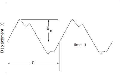
FIG. 6 Typical periodic motion.
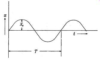
FIG. 7 Simple harmonic motion.

FIG. 8 Illustration of vibration cycles.
Harmonic Motion:
The simplest kind of periodic motion or vibration, shown in FIG. 7, is referred to as harmonic. Harmonic motions repeat each time the rotating element or machine component completes one complete cycle.
The relation between displacement and time for harmonic motion may be expressed by:
The maximum value of the displacement is X0, which is also called the amplitude.
The period, T, is usually measured in seconds; its reciprocal is the frequency of the vibration, f, measured in cycles per second (cps) or Hertz (Hz).
Another measure of frequency is the circular frequency, w, measured in radians per second. From FIG. 8, it’s clear that a full cycle of vibration (wt) occurs after 360 degrees or 2p radians (i.e., one full revolution). At this point, the function begins a new cycle.
w = 2pf For rotating machinery, the frequency is often expressed in vibrations per minute (vpm) or ...
By definition, velocity is the first derivative of displacement with respect to time. For a harmonic motion, the displacement equation is:
The first derivative of this equation gives us the equation for velocity:
This relationship tells us that the velocity is also harmonic if the displacement is harmonic and has a maximum value or amplitude of -wX0.
By definition, acceleration is the second derivative of displacement (i.e., the first derivative of velocity) with respect to time:
This function is also harmonic with amplitude of w2 X0.
Consider two frequencies given by the expression X1 = a sin(wt) and X2 = b sin(wt + f), which are shown in FIG. 9 plotted against wt as the X-axis. The quantity, f, in the equation for X2 is known as the phase angle or phase difference between the two vibrations. Because of f, the two vibrations don’t attain their maximum displacements at the same time. One is seconds behind the other. Note that these two motions have the same frequency, w. A phase angle has meaning only for two motions of the same frequency.
FIG. 9 Two harmonic motions with a phase angle between them.
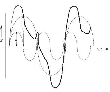
FIG. 10 Nonharmonic periodic motion.
Nonharmonic Motion:
In most machinery, there are numerous sources of vibrations; therefore, most time domain vibration profiles are nonharmonic (represented by the solid line in FIG. 10). Although all harmonic motions are periodic, not every periodic motion is harmonic. In FIG. 10, the dashed lines represent harmonic motions. FIG. 10 is the superposition of two sine waves having different frequencies. These curves are represented by the following equations:
The total vibration represented by the solid line is the sum of the dashed lines. The following equation represents the total vibration:
Any periodic function can be represented as a series of sine functions having frequencies of w, 2w, 3w, etc.:
The previous equation is known as a Fourier Series, which is a function of time or f(t). The amplitudes (A1, A2, etc.) of the various discrete vibrations and their phase angles (f1, f2, f3, . . .) can be determined mathematically when the value of function f(t) is known. Note that these data are obtained using a transducer and a portable vibration analyzer.
The terms, 2w, 3w, etc., are referred to as the harmonics of the primary frequency, w.
In most vibration signatures, the primary frequency component is one of the running speeds of the machine-train (1X or 1w). In addition, a signature may be expected to have one or more harmonics , for example, at two times (2X), three times (3X), and other multiples of the primary running speed.
Measurable Parameters
As shown previously, vibrations can be displayed graphically as plots, which are referred to as vibration profiles or signatures. These plots are based on measurable parameters (i.e., frequency and amplitude). [Note that the terms profile and signature are sometimes used interchangeably by industry. In this book, however, profile is used to refer either to time-domain (also may be called time trace or waveform) or frequency-domain plots. The term signature refers to a frequency-domain plot.]
Frequency:
Frequency is defined as the number of repetitions of a specific forcing function or vibration component over a specific unit of time. Take for example a four-spoke wheel with an accelerometer attached. Every time the shaft completes one rotation, each of the four spokes passes the accelerometer once, which is referred to as four cycles per revolution. Therefore, if the shaft rotates at 100 rotations per minute (rpm), the frequency of the spokes passing the accelerometer is 400 cycles per minute (cpm). In addition to cpm, frequency is commonly expressed in cycles per second (cps) or Hertz (Hz).
Note that for simplicity, a machine element's vibration frequency is commonly expressed as a multiple of the shaft's rotation speed. In the previous example, the frequency would be indicated as 4X, or four times the running speed. In addition, because some malfunctions tend to occur at specific frequencies, it helps to segregate certain classes of malfunctions from others.
Note, however, that the frequency/malfunction relationship is not mutually exclusive, and a specific mechanical problem cannot definitely be attributed to a unique frequency. Although frequency is a very important piece of information with regard to isolating machinery malfunctions, it’s only one part of the total picture. It’s necessary to evaluate all data before arriving at a conclusion.
Amplitude:
Amplitude refers to the maximum value of a motion or vibration. This value can be represented in terms of displacement (mils), velocity (inches per second), or acceleration (inches per second squared), each of which is discussed in more detail in the Maximum Vibration Measurement section that follows.
Amplitude can be measured as the sum of all the forces causing vibrations within a piece of machinery (broadband), as discrete measurements for the individual forces (component), or for individual user-selected forces (narrowband). Broadband, component, and narrowband are discussed in the Measurement Classifications section that follows. Also discussed in this section are the common curve elements: peak-to-peak, zero-to-peak, and root-mean-square.
Maximum Vibration Measurement. The maximum value of a vibration, or amplitude, is expressed as displacement, velocity, or acceleration. Most of the microprocessor based, frequency-domain vibration systems will convert the acquired data to the desired form. Because industrial vibration-severity standards are typically expressed in one of these terms, it’s necessary to have a clear understanding of their relationship.
Displacement. Displacement is the actual change in distance or position of an object relative to a reference point and is usually expressed in units of mils, 0.001 inch. For example, displacement is the actual radial or axial movement of the shaft in relation to the normal centerline, usually using the machine housing as the stationary reference. Vibration data, such as shaft displacement measurements acquired using a proximity probe or displacement transducer, should always be expressed in terms of mils, peak-to-peak.
Velocity. Velocity is defined as the time rate of change of displacement (i.e., the first derivative, or X.) and is usually expressed as inches per second (ips). In simple terms, velocity is a description of how fast a vibration component is moving rather than how far, which is described by displacement.
Used in conjunction with zero-to-peak (PK) terms, velocity is the best representation of the true energy generated by a machine when relative or bearing cap-data are used.
[Note: Most vibration-monitoring programs rely on data acquired from machine housing or bearing caps.] In most cases, peak velocity values are used with vibration data between 0 and 1,000Hz. These data are acquired with microprocessor-based, frequency-domain systems.
Acceleration. Acceleration is defined as the time rate of change of velocity (i.e., second derivative of displacement, or X ¨ ) and is expressed in units of inches per second squared (in/sec^2). Vibration frequencies above 1,000Hz should always be expressed as acceleration.
Acceleration is commonly expressed in terms of the gravitational constant, g, which is 32.17 ft/sec^2. In vibration-analysis applications, acceleration is typically expressed in terms of g-RMS or g-PK. These are the best measures of the force generated by a machine, a group of components, or one of its components.
Measurement Classifications. There are at least three classifications of amplitude measurements used in vibration analysis: broadband, narrowband, and component.
Broadband or overall. The total energy of all vibration components generated by a machine is reflected by broadband, or overall, amplitude measurements. The normal convention for expressing the frequency range of broadband energy is a filtered range between 10 to 10,000Hz, or 600 to 600,000 cpm. Because most vibration-severity charts are based on this filtered broadband, caution should be exercised to ensure that collected data are consistent with the charts.
Narrowband. Narrowband amplitude measurements refer to those that result from monitoring the energy generated by a user-selected group of vibration frequencies.
Generally, this amplitude represents the energy generated by a filtered band of vibration components, failure mode, or forcing functions. For example, the total energy generated by flow instability can be captured using a filtered narrowband around the vane or blade-passing frequency.
FIG. 11 Relationship of vibration amplitude. (not shown)
Component. The energy generated by a unique machine component, motion, or other forcing function can yield its own amplitude measurement. For example, the energy generated by the rotational speed of a shaft, gear set meshing, or similar machine components produces discrete vibration components whose amplitude can be measured.
Common Elements of Curves. All vibration amplitude curves, which can represent displacement, velocity, or acceleration, have common elements that can be used to describe the function. These common elements are peak-to-peak, zero-to-peak, and root-mean-square, each of which are illustrated in FIG. 11.
Peak-to-peak. As illustrated in FIG. 11, the peak-to-peak amplitude (2A, where A is the zero-to-peak) reflects the total amplitude generated by a machine, a group of components, or one of its components. This depends on whether the data gathered are broadband, narrowband, or component. The unit of measurement is useful when the analyst needs to know the total displacement or maximum energy produced by the machine's vibration profile.
Technically, peak-to-peak values should be used in conjunction with actual shaft displacement data, which are measured with a proximity or displacement transducer.
Peak-to-peak terms should not be used for vibration data acquired using either relative vibration data from bearing caps or when using a velocity or acceleration transducer. The only exception is when vibration levels must be compared to vibration-severity charts based on peak-to-peak values.
Zero-to-peak. Zero-to-peak (A), or simply peak, values are equal to one half of the peak-to-peak value. In general, relative vibration data acquired using a velocity transducer are expressed in terms of peak.
Root-mean-square. Root-mean-square (RMS) is the statistical average value of the amplitude generated by a machine, one of its components, or a group of components.
Referring to FIG. 11, RMS is equal to 0.707 of the zero-to-peak value, A. Normally, RMS data are used in conjunction with relative vibration data acquired using an accelerometer or expressed in terms of acceleration.
MACHINE DYNAMICS
The primary reasons for vibration-profile variations are the dynamics of the machine, which are affected by mass, stiffness, damping, and degrees of freedom; however, care must be taken because the vibration profile and energy levels generated by a machine may vary depending on the location and orientation of the measurement.
Mass, Stiffness, and Damping
The three primary factors that determine the normal vibration energy levels and the resulting vibration profiles are mass, stiffness, and damping. Every machine-train is designed with a dynamic support system that is based on the following: the mass of the dynamic component(s), specific support system stiffness, and a specific amount of damping.
Mass:
Mass is the property that describes how much material is present. Dynamically, the property describes how an unrestricted body resists the application of an external force. Simply stated, the greater the mass, the greater the force required to accelerate it. Mass is obtained by dividing the weight of a body (e.g., rotor assembly) by the local acceleration of gravity, g.
The English system of units is complicated compared to the metric system. In the English system, the units of mass are pounds-mass (lbm) and the units of weight are pounds-force (lbf). By definition, a weight (i.e., force) of one lbf equals the force produced by one lbm under the acceleration of gravity. Therefore, the constant, gc, which has the same numerical value as g (32.17) and units of lbm-ft/lbf-sec^2 , is used in the definition of weight: Mass Weight lbf ft lbm ft, lbf
Stiffness:
Stiffness is a spring-like property that describes the level of resisting force that results when a body changes in length. Units of stiffness are often given as pounds per inch (lbf/in). Machine-trains have three stiffness properties that must be considered in vibration analysis: shaft stiffness, vertical stiffness, and horizontal stiffness.
Shaft Stiffness. Most machine-trains used in industry have flexible shafts and relatively long spans between bearing-support points. As a result, these shafts tend to flex in normal operation. Three factors determine the amount of flex and mode shape that these shafts have in normal operation: shaft diameter, shaft material properties, and span length. A small-diameter shaft with a long span will obviously flex more than one with a larger diameter or shorter span.
Vertical Stiffness. The rotor-bearing support structure of a machine typically has more stiffness in the vertical plane than in the horizontal plane. Generally, the structural rigidity of a bearing-support structure is much greater in the vertical plane. The full weight of and the dynamic forces generated by the rotating element are fully sup ported by a pedestal cross-section that provides maximum stiffness.
In typical rotating machinery, the vibration profile generated by a normal machine contains lower amplitudes in the vertical plane. In most cases, this lower profile can be directly attributed to the difference in stiffness of the vertical plane when compared to the horizontal plane.
Horizontal Stiffness. Most bearing pedestals have more freedom in the horizontal direction than in the vertical. In most applications, the vertical height of the pedestal is much greater than the horizontal cross-section. As a result, the entire pedestal can flex in the horizontal plane as the machine rotates.
This lower stiffness generally results in higher vibration levels in the horizontal plane.
This is especially true when the machine is subjected to abnormal modes of operation or when the machine is unbalanced or misaligned.
Damping:
Damping is a means of reducing velocity through resistance to motion, in particular by forcing an object through a liquid or gas, or along another body. Units of damping are often given as pounds per inch per second (lbf/in/sec, which is also expressed as lbf-sec/in).
The boundary conditions established by the machine design determine the freedom of movement permitted within the machine-train. A basic understanding of this concept is essential for vibration analysis. Free vibration refers to the vibration of a damped (as well as undamped) system of masses with motion entirely influenced by their potential energy. Forced vibration occurs when motion is sustained or driven by an applied periodic force in either damped or undamped systems. The following sections discuss free and forced vibration for both damped and undamped systems.
Free Vibration-Undamped. To understand the interactions of mass and stiffness, consider the case of undamped free vibration of a single mass that only moves vertically, which is illustrated in FIG. 12. In this figure, the mass "M" is sup ported by a spring that has a stiffness "K" (also referred to as the spring constant), which is defined as the number of pounds tension necessary to extend the spring one inch.
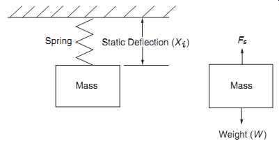
FIG. 12 Undamped spring-mass system.
The force created by the static deflection, Xi, of the spring supports the weight, W, of the mass. Also included in FIG. 12 is the free-body diagram that illustrates the two forces acting on the mass. These forces are the weight (also referred to as the inertia force) and an equal, yet opposite force that results from the spring (referred to as the spring force, Fs).
The relationship between the weight of mass, M, and the static deflection of the spring can be calculated using the following equation:
W = KXi
If the spring is displaced downward some distance, X0, from Xi and released, it will oscillate up and down. The force from the spring, Fs, can be written as follows, where "a" is the acceleration of the mass:
It’s common practice to replace acceleration, a, with the second derivative of the displacement, X, of the mass with respect to time, t. Making this substitution, the equation that defines the motion of the mass can be expressed as:
Motion of the mass is known to be periodic. Therefore, the displacement can be described by the expression:
Where:
X = Displacement at time t X0 = Initial displacement of the mass w = Frequency of the oscillation (natural or resonant frequency) t = Time
If this equation is differentiated and the result inserted into the equation that defines motion, the natural frequency of the mass can be calculated. The first derivative of the equation for motion yields the equation for velocity. The second derivative of the equation yields acceleration.
Inserting the expression for acceleration, or into the equation for Fs yields the following:
Solving this expression for w yields the equation:
Where:
w = Natural frequency of mass
K = Spring constant
M = Mass
Note that, theoretically, undamped free vibration persists forever; however, this never occurs in nature, and all free vibrations die down after time because of damping, which is discussed in the next section.
Free Vibration-Damped. A slight increase in system complexity results when a damping element is added to the spring-mass system shown in FIG. 13. This type of damping is referred to as viscous damping. Dynamically, this system is the same as the undamped system illustrated in FIG. 12, except for the damper, which usually is an oil or air dashpot mechanism. A damper is used to continuously decrease the velocity and the resulting energy of a mass undergoing oscillatory motion.
The system consists of the inertia force caused by the mass and the spring force, but a new force is introduced. This force is referred to as the damping force and is proportional to the damping constant, or the coefficient of viscous damping, c. The damping force is also proportional to the velocity of the body and, as it’s applied, it opposes the motion at each instant.
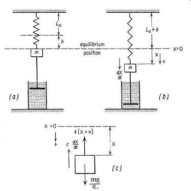
FIG. 13 Damped spring-mass system.
In FIG. 13, the non-elongated length of the spring is "Lo" and the elongation caused by the weight of the mass is expressed by "h." Therefore, the weight of the mass is Kh. Part (a) of FIG. 13 shows the mass in its position of stable equilibrium. Part (b) shows the mass displaced downward a distance X from the equilibrium position.
Note that X is considered positive in the downward direction.
Part (c) of FIG. 13 is a free-body diagram of the mass, which has three forces acting on it. The weight (Mg/gc), which is directed downward, is always positive. The damping force which is the damping constant times velocity, acts opposite to the direction of the velocity. The spring force, K(X + h), acts in the direction opposite to the displacement. Using Newton's equation of motion, where SF = Ma, the sum of the forces acting on the mass can be represented by the following equation, remembering that X is positive in the downward direction:
In order to look up the solution to the above equation in a differential equations table (such as in CRC Handbook of Chemistry and Physics), it’s necessary to change the form of this equation. This can be accomplished by defining the relationships, cgc/M = 2m and Kg /M = w2, which converts the equation to the following form:
This shows that free vibration is periodic and is the solution for X. For damped free vibration, however, the damping constant, c, is not zero.
There are different conditions of damping: critical, overdamping, and underdamping.
Critical damping occurs when m equals w. Overdamping occurs when m is greater than w. Underdamping occurs when m is less than w.
The only condition that results in oscillatory motion and, therefore, represents a mechanical vibration is underdamping. The other two conditions result in periodic motions. When damping is less than critical (m < w), then the following equation applies:
In undamped forced vibration, the only difference in the equation for undamped free vibration is that instead of the equation being equal to zero, it’s equal to F0 sin(wt):
Because the spring is not initially displaced and is "driven" by the function F0 sin(wt), a particular solution, X = X0 sin(wt), is logical. Substituting this solution into the above equation and performing mathematical manipulations yields the following equation for X:
X = Spring displacement at time, t Xst = Static spring deflection under constant load, F0 w = Forced frequency wn = Natural frequency of the oscillation t = Time; C1 and C2 = Integration constants determined from specific boundary conditions
In the above equation, the first two terms are the undamped free vibration, whereas the third term is the undamped forced vibration. The solution, containing the sum of two sine waves of different frequencies, is not a harmonic motion.
Forced Vibration-Damped. In a damped forced vibration system such as the one shown in FIG. 14, the motion of the mass "M" has two parts: (1) the damped free vibration at the damped natural frequency and (2) the steady-state harmonic motions at the forcing frequency. The damped natural frequency component decays quickly, but the steady-state harmonic associated with the external force remains as long as the energy force is present.
With damped forced vibration, the only difference in its equation and the equation for damped free vibration is that it’s equal to F0 sin(wt) as shown below instead of being equal to zero.
With damped vibration, the damping constant, "c," is not equal to zero and the solution of the equation becomes complex assuming the function, X = X0 sin(wt - f). In
Forced Vibration-Undamped. The simple systems described in the preceding two sections on free vibration are alike in that they are not forced to vibrate by any exciting force or motion. Their major contribution to the discussion of vibration fundamentals is that they illustrate how a system's natural or resonant frequency depends on the mass, stiffness, and damping characteristics.
The mass-stiffness-damping system also can be disturbed by a periodic variation of external forces applied to the mass at any frequency. The system shown in FIG. 12 is increased in complexity by adding an external force, F0, acting downward on the mass.
this equation, f is the phase angle, or the number of degrees that the external force, F0 sin(wt), is ahead of the displacement, X0 sin(wt - f). Using vector concepts, the following equations apply, which can be solved because there are two equations and two unknowns:
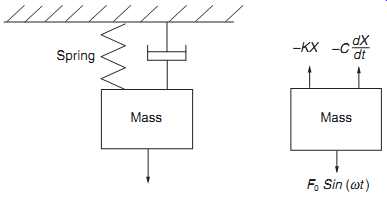
FIG. 14 Damped forced vibration system.
Vertical vector component:
Horizontal vector component:
For damped forced vibrations, three different frequencies have to be distinguished: the undamped natural frequency, the damped natural frequency, and the frequency of maximum forced amplitude, sometimes referred to as the resonant frequency.
Degrees of Freedom
In a mechanical system, the degrees of freedom indicate how many numbers are required to express its geometrical position at any instant. In machine-trains, the relationship of mass, stiffness, and damping is not the same in all directions. As a result, the rotating or dynamic elements within the machine move more in one direction than in another. A clear understanding of the degrees of freedom is important because it has a direct impact on the vibration amplitudes generated by a machine or process system.
One Degree of Freedom:
If the geometrical position of a mechanical system can be defined or expressed as a single value, the machine is said to have one degree of freedom. For example, the position of a piston moving in a cylinder can be specified at any point in time by measuring the distance from the cylinder end.
A single degree of freedom is not limited to simple mechanical systems such as the cylinder. For example, a 12-cylinder gasoline engine with a rigid crankshaft and a rigidly mounted cylinder block has only one degree of freedom. The position of all its moving parts (i.e., pistons, rods, valves, cam shafts) can be expressed by a single value. In this instance, the value would be the angle of the crankshaft; however, when mounted on flexible springs, this engine has multiple degrees of freedom. In addition to the movement of its internal parts in relationship to the crank, the entire engine can now move in any direction. As a result, the position of the engine and any of its internal parts requires more than one value to plot its actual position in space.
The definitions and relationships of mass, stiffness, and damping in the preceding section assumed a single degree of freedom. In other words, movement was limited to a single plane. Therefore, the formulas are applicable for all single-degree-of freedom mechanical systems.
The calculation for torque is a primary example of a single degree of freedom in a mechanical system. FIG. 15 represents a disk with a moment of inertia, I, that is attached to a shaft of torsional stiffness, k.
Torsional stiffness is defined as the externally applied torque, T, in inch-pounds needed to turn the disk one radian (57.3 degrees). Torque can be represented by the following equations:
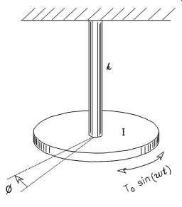
FIG. 15 Torsional one-degree-of freedom system.
In this example, three torques are acting on the disk: the spring torque, the damping torque (caused by the viscosity of the air), and the external torque. The spring torque is minus (-) kf where f is measured in radians. The damping torque is minus (-) cf, where "c" is the damping constant. In this example, "c" is the damping torque on the disk caused by an angular speed of rotation of one radian per second. The external torque is T0 sin (wt).
Two Degrees of Freedom:
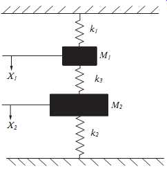
FIG. 16 Undamped two-degrees of-freedom system with a spring couple.
The theory for a one-degree-of-freedom system is useful for determining resonant or natural frequencies that occur in all machine-trains and process systems; however, few machines have only one degree of freedom. Practically, most machines will have two or more degrees of freedom. This section provides a brief overview of the theories associated with two degrees of freedom. An undamped two-degree-of-freedom system is illustrated in FIG. 16.
This diagram consists of two masses, M1 and M2, that are suspended from springs, K1 and K2. The two masses are tied together, or coupled, by spring, K3, so that they are forced to act together. In this example, the movement of the two masses is limited to the vertical plane and, therefore, horizontal movement can be ignored. As in the single degree-of-freedom examples, the absolute position of each mass is defined by its vertical position above or below the neutral, or reference, point. Because there are two coupled masses, two locations (i.e., one for M1 and one for M2) are required to locate the absolute position of the system.
To calculate the free or natural modes of vibration, note that two distinct forces are acting on mass, M1: the force of the main spring, K1, and that of the coupling spring, K3. The main force acts upward and is defined as -K1X1. The shortening of the coupling spring is equal to the difference in the vertical position of the two masses, X1 - X2. Therefore, the compressive force of the coupling spring is K3(X1 - X2). The com pressed coupling spring pushes the top mass, M1, upward so that the force is negative.
Because these are the only tangible forces acting on M1, the equation of motion for the top mass can be written as:
The equation of motion for the second mass, M2, is derived in the same manner. To make it easier to understand, turn the figure upside down and reverse the direction of X1 and X2. The equation then becomes:
If we assume that the masses, M1 and M2, undergo harmonic motions with the same frequency, w, and with different amplitudes, A1 and A2, their behavior can be represented as:
By substituting these into the differential equations, two equations for the amplitude ratio, can be found:
For a solution of the form we assumed to exist, these two equations must be equal:
This equation, known as the frequency equation, has two solutions for w^2 . When substituted in either of the preceding equations, each one of these gives a definite value for . This means that there are two solutions for this example, which are of the form A1 sin(wt) and A2 sin(wt). As with many such problems, the final answer is the super position of the two solutions with the final amplitudes and frequencies determined by the boundary conditions.
Many Degrees of Freedom:
When the number of degrees of freedom becomes greater than two, no critical new parameters enter into the problem. The dynamics of all machines can be understood by following the rules and guidelines established in the one- and two-degree(s)-of freedom equations. There are as many natural frequencies and modes of motion as there are degrees of freedom.