AMAZON multi-meters discounts AMAZON oscilloscope discounts
.Effective performance of any manufacturing or process plant depends on reliability systems that continuously operate at their best design performance levels. To achieve and sustain this performance level, the plant must have an effective way to constantly monitor and evaluate these critical systems. Operating dynamics analysis provides a cost-effective means of accomplishing this fundamental requirement.
The focus of an operating dynamics analysis program is on the manufacturing process and production systems that generate plant capacity. It’s not a maintenance management tool like traditional predictive maintenance programs. Because of perceived restrictions, such as low speed and machine complexity, of the technologies, most traditional predictive maintenance programs ignore or omit these critical systems.
Although there may be some benefit in monitoring auxiliary equipment, maximum benefit can be achieved only when reliability of the plant's critical production systems is maintained. Within the operating dynamics concept, auxiliary equipment is not ignored, but the focus is on those systems that produce capacity and revenue for the plant.
IT'S NOT PREDICTIVE MAINTENANCE
Prevention of catastrophic failure, the primary focus of predictive maintenance, is important, but programs that are restricted to this one goal won’t improve equipment reliability, nor will they provide sufficient benefits to justify their continuance.
By shifting the focus to a plant optimization tool that concentrates on capacity and reliability improvements, an operating dynamics program can greatly improve benefits to the company.
Predictive maintenance technologies can, and should, be used as a total-plant performance tool. When used correctly, these tools can provide the means to eliminate most of the factors that limit plant performance. To achieve this expanded role, the predictive maintenance program must be developed with clear goals and objectives that permit maximum utilization of the technologies. The program must be able to cross organizational boundaries and not be limited to the maintenance function. Every function within the plant affects equipment reliability and performance, and the predictive maintenance program must address all of these influences.
Vibration monitoring and analysis is the most common of the predictive maintenance technologies. It’s also the most underutilized of these tools. Most vibration-based predictive maintenance programs use less than 1 percent of the power this technology provides. The primary deficiencies of traditional predictive maintenance are:
- Technology limitations
- Limitation to maintenance issues
- Influence of process variables
- Training limitations
- Interpreting operating dynamics
Technology Limitations
Most predictive maintenance programs are severely restricted to a small population of plant equipment and systems. For example, vibration-based programs are generally restricted to simple, rotating machinery, such as fans, pumps, or compressors. Thermography is typically restricted to electrical switchgear and related electrical equipment. These restrictions are thought to be physical limitations of the predictive technologies. In truth, they are not.
Predictive instrumentation has the ability to effectively acquire accurate data from almost any manufacturing or process system. Restrictions, such as low speed, are purely artificial. Not only can many of the vibration meters record data at low speeds, but they can also be used to acquire most process variables, such as temperature, pressure, or flow. Because most have the ability to convert any proportional electrical signal into user-selected engineering units, they are in fact multimeters that can be used as part of a comprehensive process performance analysis program.
Limitation to Maintenance Issues
From its inception, predictive maintenance has been perceived as a maintenance improvement tool. Its sole purpose was, and is, to prevent catastrophic failure of plant equipment. Although it’s capable of providing the diagnostic data required to meet this goal, limiting these technologies solely to this task won’t improve overall plant performance.
When predictive programs are limited to the traditional maintenance function, they must ignore those issues or contributors that directly affect equipment reliability.
Outside factors, such as poor operating practices, are totally ignored.
Many predictive maintenance programs are limited to simple trending of vibration, infrared, or lubricating oil data. The perception that a radical change in the relative values indicates a corresponding change in equipment condition is valid; however, this logic does not go far enough. The predictive analyst must understand the true meaning of a change in one or more of these relative values. If a compressor's vibration level doubles, what does the change really mean? It may mean that serious mechanical damage has occurred, but it could simply mean that the compressor's load was reduced.
A machine or process system is much like the human body. It generates a variety of signals, like a heartbeat, that define its physical condition. In a traditional predictive maintenance program, the analyst evaluates one or a few of these signals as part of his or her determination of condition. For example, the analyst may examine the vibration profile or heartbeat of the machine. Although this approach has some merit, it cannot provide a complete understanding of the machine or the system's true operating condition.
When a doctor evaluates a patient, he or she uses all of the body's signals to diagnose an illness. Instead of relying on the patient's heartbeat, the doctor also uses a variety of blood tests, temperature, urine composition, brainwave patterns, and a variety of other measurements of the body's condition. In other words, the doctor uses all of the measurable indices of the patient's condition. These data are then compared to the benchmark or normal profile for the human body.
Operating dynamics is much like the physician's approach. It uses all of the indices that quantify the operating condition of a machine-train or process system and evaluates them using a design benchmark that defines normal for the system.
Influence of Process Variables
In many cases, the vibration-monitoring program isolates each machine-train or a component of a machine-train and ignores its system. This approach results in two major limitations: it ignores (1) the efficiency or effectiveness of the machine-train and (2) the influence of variations in the process.
When the diagnostic logic is limited to common failure modes, such as imbalance, misalignment, and so on, the benefits derived from vibration analyses are severely restricted. Diagnostic logic should include the total operating effectiveness and efficiency of each machine-train as a part of its total system. For example, a centrifugal pump is installed as part of a larger system. Its function is to reliably deliver, with the lowest operating costs, a specific volume of liquid and a specific pressure to the larger system. Few programs consider this fundamental requirement of the pump. Instead, their total focus is on the mechanical condition of the pump and its driver.
The second limitation to many vibration programs is that the analyst ignores the influence of the system on a machine-train's vibration profile. All machine-trains are affected by system variations, no matter how simple or complex. For example, a comparison of vibration profiles acquired from a centrifugal compressor operating at 100 percent load and at 50 percent load will clearly be different. The amplitude of all rotational frequency components will increase by as much as four times at 50 percent load. Why? Simply because more freedom of movement occurs at the lower load.
As part of the compressor design, load was used to stabilize the rotor. The designer balanced the centrifugal and centripetal forces within the compressor based on the design load (100 percent). When the compressor is operated at reduced or excessive loads, the rotor becomes unbalanced because the internal forces are no longer equal.
In addition, the spring constant of the rotor-bearing support structure also changes with load: It becomes weaker as load is reduced and stronger as it’s increased.
In more complex systems, such as paper mills other continuous process lines, the impact of the production process is much more severe. The variation in incoming product, line speeds, tensions, and a variety of other variables directly impacts the operating dynamics of the system and all of its components. The vibration profiles generated by these system components also vary with the change in the production variables. The vibration analyst must adjust for these changes before the technology can be truly beneficial as either a maintenance scheduling or plant improvement tool.
Because most predictive maintenance programs are established as maintenance tools, they ignore the impact of operating procedures and practices on the dynamics of system components. Variables such as ramp rate, startup and shutdown practices, and an infinite variety of other operator-controlled variables have a direct impact on both reliability and the vibration profiles generated by system components. It’s difficult, if not impossible, to accurately detect, isolate, and identify incipient problems without clearly understanding these influences. The predictive maintenance program should evaluate existing operating practices; quantify their impact on equipment reliability, effectiveness, and costs; and provide recommended modifications to these practices that will improve overall performance of the production system.
Training Limitations
In general, predictive maintenance analysts receive between 5 and 25 days of training as part of the initial startup cost. This training is limited to three to five days of predictive system training by the system vendor and about five days of vibration or infrared technology training. In too many cases, little additional training is provided.
Analysts are expected to teach themselves or network with other analysts to master their trade. This level of training is not enough to gain even minimal benefits from predictive maintenance.
Vendor training is usually limited to use of the system and provides little, if any, practical technology training. The technology courses that are currently available are of limited value. Most are limited to common failure modes and don’t include any training in machine design or machine dynamics. Instead, analysts are taught to identify simple failure modes of generic machine-trains.
To be effective, predictive analysts must have a thorough knowledge of machine/ system design and machine dynamics. This knowledge provides the minimum base required to effectively use predictive maintenance technologies. Typically, a graduate mechanical engineer can master this basic knowledge of machine design, machine dynamics, and proper use of predictive tools in about 13 weeks of classroom training.
Non-engineers, with good mechanical aptitude, will need 26 or more weeks of formal training.
Understanding Machine Dynamics
It Starts with the Design:
Every machine or process system is designed to perform a specific function or range of functions. To use operating dynamics analysis, one must first fully understand how machines and process systems perform their work. This understanding must start with a thorough design review that identifies the criteria that were used to design a machine and its installed system. In addition, the analyst must also understand the inherent weaknesses and potential failure modes of these systems. For example, consider the centrifugal pump.
====
INLINE CONFIGURATION 100 PSID 100 PSID 300 PSI 100 PSI 100 PSI 100 PSID 100 PSID 100 PSID OPPOSED CONFIGURATION
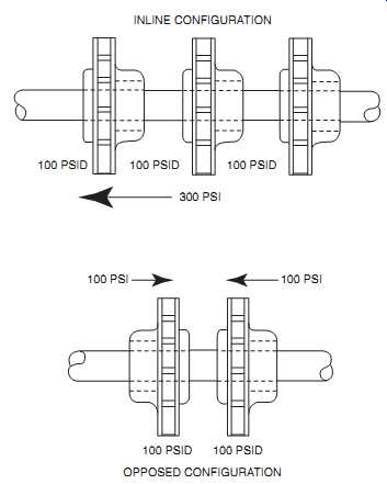
FIG. 1 Impeller orientation.
====
Centrifugal pumps are highly susceptible to variations in process parameters, such as suction pressure, specific gravity of the pumped liquid, back-pressure induced by control valves, and changes in demand volume. Therefore, the dominant reasons for centrifugal pump failures are usually process related.
Several factors dominate pump performance and reliability: internal configuration, suction condition, total dynamic pressure or head, hydraulic curve, brake horsepower, installation, and operating methods. These factors must be understood and used to evaluate any centrifugal pump-related problem or event.
All centrifugal pumps are not alike. Variations in the internal configuration occur in the impeller type and orientation. These variations have a direct impact on a pump's stability, useful life, and performance characteristics.
There are a variety of impeller types used in centrifugal pumps. They range from simple radial-flow, open designs to complex variable-pitch, high-volume enclosed designs. Each of these types is designed to perform a specific function and should be selected with care. In relatively small, general-purpose pumps, the impellers are normally designed to provide radial flow, and the choices are limited to either enclosed or open design.
Enclosed impellers are cast with the vanes fully encased between two disks. This type of impeller is generally used for clean, solid-free liquids. It has a much higher efficiency than the open design. Open impellers have only one disk, and the opposite side of the vanes is open to the liquid. Because of its lower efficiency, this design is limited to applications where slurries or solids are an integral part of the liquid.
In single-stage centrifugal pumps, impeller orientation is fixed and is not a factor in pump performance; however, it must be carefully considered in multistage pumps, which are available in two configurations: inline and opposed.
Inline configurations (see FIG. 1) have all impellers facing in the same direction. As a result, the total differential pressure between the discharge and inlet is axially applied to the rotating element toward the outboard bearing. Because of this configuration, inline pumps are highly susceptible to changes in the operating envelope.
Because of the tremendous axial pressures that are created by the inline design, these pumps must have a positive means of limiting endplay, or axial movement, of the rotating element. Normally, one of two methods is used to fix or limit axial movement: (1) a large thrust bearing is installed at the outboard end of the pump to restrict movement, or (2) discharge pressure is vented to a piston mounted on the outboard end of the shaft.
Multistage pumps that use opposed impellers are much more stable and can tolerate a broader range of process variables than those with an inline configuration. In the opposed-impeller design, sets of impellers are mounted back-to-back on the shaft. As a result, the other cancels the thrust or axial force generated by one of the pairs. This design approach virtually eliminates axial forces. As a result, the pump does not require a massive thrust-bearing or balancing piston to fix the axial position of the shaft and rotating element.
Because the axial forces are balanced, this type of pump is much more tolerant of changes in flow and differential pressure than the inline design; however, it’s not immune to process instability or to the transient forces caused by frequent radical changes in the operating envelope.
Factors that Determine Performance:
Centrifugal pump performance is primarily controlled by two variables: suction conditions and total system pressure or head requirement. Total system pressure consist of the total vertical lift or elevation change, friction losses in the piping, and flow restrictions caused by the process. Other variables affecting performance include the pump's hydraulic curve and brake horsepower.
Suction Conditions. Factors affecting suction conditions are the net positive suction head, suction volume, and entrained air or gas. Suction pressure, called net positive suction head (NPSH), is one of the major factors governing pump performance. The variables affecting suction head are shown in FIG. 2.
Centrifugal pumps must have a minimum amount of consistent and constant positive pressure at the eye of the impeller. If this suction pressure is not available, the pump will be unable to transfer liquid. The suction supply can be open and below the pump's centerline, but the atmospheric pressure must be greater than the pressure required to lift the liquid to the impeller eye and to provide the minimum NPSH required for proper pump operation.
At sea level, atmospheric pressure generates a pressure of 14.7 pounds per square inch (psi) to the surface of the supply liquid. This pressure minus vapor pressure, friction loss, velocity head, and static lift must be enough to provide the minimum NPSH requirements of the pump. These requirements vary with the volume of liquid transferred by the pump.
Most pump curves provide the minimum NPSH required for various flow conditions.
This information, which is usually labeled NPSHR, is generally presented as a rising curve located near the bottom of the hydraulic curve. The data are usually expressed in "feet of head" rather than psi.
The pump's supply system must provide a consistent volume of single-phase liquid equal to or greater than the volume delivered by the pump. To accomplish this, the suction supply should have relatively constant volume and properties (e.g., pressure, temperature, specific gravity). Special attention must be paid to applications where the liquid has variable physical properties (e.g., specific gravity, density, viscosity).
As the suction supply's properties vary, effective pump performance and reliability will be adversely affected.
===
(Hvp) VAPOR PRESSURE (Hf) FRICTION LOSS IN SUCTION VELOCITY HEAD LOSS AT IMPELLER USEFUL PRESSURE AVAILABLE N.P.S.H. LOSS DUE TO USEFUL PRESSURE AT SURFACE OF LIQUID ATMOSPHERIC PRESSURE AT SURFACE OF LIQUID STATIC LIFT
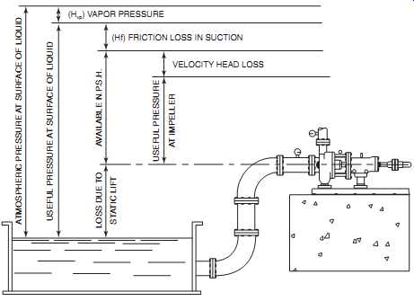
FIG. 2 Net positive suction head requirements.
===
In applications where two or more pumps operate within the same system, special attention must be given to the suction flow requirements. Generally, these applications can be divided into two classifications: pumps in series and pumps in parallel.
Most pumps are designed to handle single-phase liquids within a limited range of specific gravity or viscosity. Entrainment of gases, such as air or steam, has an adverse effect on both the pump's efficiency and its useful operating life. This is one form of cavitation, which is a common failure mode of centrifugal pumps. The typical causes of cavitation are leaks in suction piping and valves or a change of phase induced by liquid temperature or suction pressure deviations. For example, a one-pound suction pressure change in a boiler-feed application may permit the de-aerator-supplied water to flash into steam. The introduction of a two-phase mixture of hot water and steam into the pump causes accelerated wear, instability, loss of pump performance, and chronic failure problems.
Total System Head. Centrifugal pump performance is controlled by the total system head (TSH) requirement, unlike positive-displacement pumps. TSH is defined as the total pressure required to overcome all resistance at a given flow. This value includes all vertical lift, friction loss, and back-pressure generated by the entire system. It deter mines the efficiency, discharge volume, and stability of the pump.
===
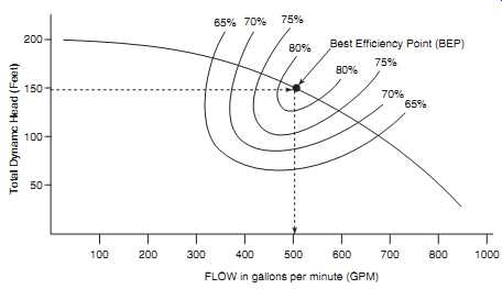
FIG. 3 Simple hydraulic curve for centrifugal pump. FLOW in gallons
per minute (GPM; Total Dynamic Head (Feet)
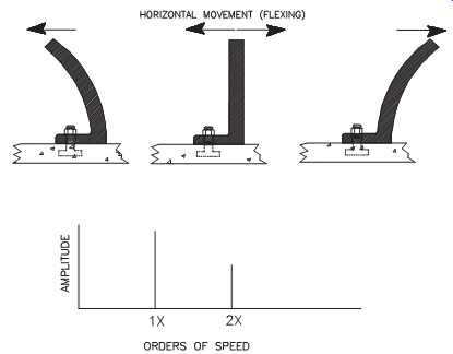
FIG. 4 Actual centrifugal pump performance depends on total system
head. FLOW in gallons per minute (GPM)
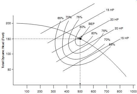
FIG. 5 Brake horsepower needs to change with process parameters.
===
Total Dynamic Head. Total dynamic head (TDH) is the difference between the discharge and suction pressure of a centrifugal pump. Pump manufacturers that generate hydraulic curves, such as those shown in FIGS. 3, 4, and 5, use this value.
These curves represent the performance that can be expected for a particular pump under specific operating conditions. For example, a pump with a discharge pressure of 100 psig and a positive pressure of 10 psig at the suction will have a TDH of 90 psig.
Most pump hydraulic curves define pressure to be TDH rather than actual discharge pressure. This consideration is important when evaluating pump problems. For example, a variation in suction pressure has a measurable impact on both discharge pressure and volume. FIG. 3 is a simplified hydraulic curve for a single-stage centrifugal pump. The vertical axis is TDH, and the horizontal axis is discharge volume or flow.
The best operating point for any centrifugal pump is called the best efficiency point (BEP). This is the point on the curve where the pump delivers the best combination of pressure and flow. In addition, the BEP defines the point that provides the most stable pump operation with the lowest power consumption and longest maintenance free service life.
In any installation, the pump will always operate at the point where its TDH equals the TSH. When selecting a pump, it’s hoped that the BEP is near the required flow where the TDH equals TSH on the curve. If it’s not, some operating-cost penalty will result from the pump's inefficiency. This is often unavoidable because pump selection is determined by choosing from what is available commercially as opposed to selecting one that would provide the best theoretical performance.
For the centrifugal pump illustrated in FIG. 3, the BEP occurs at a flow of 500 gallons per minute with 150 feet TDH. If the TSH were increased to 175 feet, however, the pump's output would decrease to 350 gallons per minute. Conversely, a decrease in TSH would increase the pump's output. For example, a TSH of 100 feet would result in a discharge flow of almost 670 gallons per minute.
From an operating dynamic standpoint, a centrifugal pump becomes more and more unstable as the hydraulic point moves away from the BEP. As a result, the normal service life decreases and the potential for premature failure of the pump or its components increases. A centrifugal pump should not be operated outside the efficiency range shown by the bands on its hydraulic curve, or 65 percent for the example shown in FIG. 3.
If the pump is operated to the left of the minimum recommended efficiency point, it may not discharge enough liquid to dissipate the heat generated by the pumping operation. This can result in a heat buildup within the pump that can result in catastrophic failure. This operating condition, which is called shut-off, is a leading cause of pre mature pump failure.
When the pump operates to the right of the last recommended efficiency point, it tends to overspeed and become extremely unstable. This operating condition, which is called run-out, can also result in accelerated wear and premature failure.
Brake horsepower (BHP) refers to the amount of motor horsepower required for proper pump operation. The hydraulic curve for each type of centrifugal pump reflects its performance (i.e., flow and head) at various BHPs. FIG. 5 is an example of a simplified hydraulic curve that includes the BHP parameter.
Note the diagonal lines that indicate the BHP required for various process conditions.
For example, the pump illustrated in FIG. 2 requires 22.3 horsepower at its BEP.
If the TSH required by the application increases from 150 feet to 175 feet, the horse power required by the pump increases to 24.6. Conversely, when the TSH decreases, the required horsepower also decreases.
The brake horsepower required by a centrifugal pump can be easily calculated by:
With two exceptions, the certified hydraulic curve for any centrifugal pump provides the data required by calculating the actual brake horsepower. Those exceptions are specific gravity and TDH.
Brake Horsepower = Flow GPM Specific Gravity
Total Dynamic Head Feet / 3960 x Efficiency
Specific gravity must be determined for the specific liquid being pumped. For example, water has a specific gravity of 1.0. Most other clear liquids have a specific gravity of less than 1.0. Slurries and other liquids that contain solids or are highly viscous materials generally have a higher specific gravity. Reference books, like Ingersoll Rand's Cameron's Hydraulics Databook, provide these values for many liquids.
The TDH can be directly measured for any application using two calibrated pressure gauges. Install one gauge in the suction inlet of the pump and the other on the discharge. The difference between these two readings is TDH.
With the actual TDH, flow can be determined directly from the hydraulic curve.
Simply locate the measured pressure on the hydraulic curve by drawing a horizontal line from the vertical axis (i.e., TDH) to a point where it intersects the curve. From the intersect point, draw a vertical line downward to the horizontal axis (i.e., flow).
This provides an accurate flowrate for the pump. The intersection point also provides the pump's efficiency for that specific point. Because the intersection may not fall exactly on one of the efficiency curves, some approximation may be required.
Installation:
Centrifugal pump installation should follow Hydraulic Institute Standards, which provide specific guidelines to prevent distortion of the pump and its baseplate. Distortions can result in premature wear, loss of performance, or catastrophic failure. The following should be evaluated as part of a root-cause failure analysis: foundation, piping support, and inlet and discharge piping configurations.
Centrifugal pumps require a rigid foundation that prevents torsional or linear movement of the pump and its baseplate. In most cases, this type of pump is mounted on a concrete pad with enough mass to securely support the baseplate, which has a series of mounting holes. Depending on size, there may be three to six mounting points on each side.
The baseplate must be securely bolted to the concrete foundation at all of these points.
One common installation error is to leave out the center baseplate lag bolts. This permits the baseplate to flex with the torsional load generated by the pump.
Pipe strain causes the pump casing to deform and results in premature wear and/or failure. Therefore, both suction and discharge piping must be adequately supported to prevent strain. In addition, flexible isolator connectors should be used on both suction and discharge pipes to ensure proper operation.
Centrifugal pumps are highly susceptible to turbulent flow. The Hydraulic Institute provides guidelines for piping configurations that are specifically designed to ensure laminar flow of the liquid as it enters the pump. As a general rule, the suction pipe should provide a straight, unrestricted run that is six times the inlet diameter of the pump.
Installations that have sharp turns, shut-off or flow-control valves, or undersized pipe on the suction side of the pump are prone to chronic performance problems. Such deviations from good engineering practices result in turbulent suction flow and cause hydraulic instability that severely restricts pump performance.
The restrictions on discharge piping are not as critical as for suction piping, but using good engineering practices ensures longer life and trouble-free operation of the pump.
The primary considerations that govern discharge piping design are friction losses and total vertical lift or elevation change. The combination of these two factors is called TSH, which represents the total force that the pump must overcome to perform properly. If the system is designed properly, the discharge pressure of the pump will be slightly higher than the TSH at the desired flowrate.
In most applications, it’s relatively straightforward to confirm the total elevation change of the pumped liquid. Measure all vertical rises and drops in the discharge piping, then calculate the total difference between the pump's centerline and the final delivery point.
Determining the total friction loss, however, is not as simple. Friction loss is caused by several factors, all of which depend on the flow velocity generated by the pump.
The major sources of friction loss include:
• Friction between the pumped liquid and the sidewalls of the pipe
• Valves, elbows, and other mechanical flow restrictions
• Other flow restrictions, such as back-pressure created by the weight of liquid in the delivery storage tank or resistance within the system component that uses the pumped liquid.
Several reference books, like Ingersoll-Rand's Cameron's Hydraulics Databook, provide the pipe-friction losses for common pipes under various flow conditions.
Generally, data tables define the approximate losses in terms of specific pipe lengths or runs. Friction loss can be approximated by measuring the total run length of each pipe size used in the discharge system, dividing the total by the equivalent length used in the table, and multiplying the result by the friction loss given in the table.
Each time the flow is interrupted by a change of direction, a restriction caused by valving, or a change in pipe diameter, the flow resistance of the piping increases substantially. The actual amount of this increase depends on the nature of the restriction.
For example, a short-radius elbow creates much more resistance than a long-radius elbow; a ball valve's resistance is much greater than a gate valve's; and the resistance from a pipe-size reduction of four inches will be greater than for a one-inch reduction. Reference tables are available in hydraulics handbooks that provide the relative values for each of the major sources of friction loss. As in the friction tables mentioned earlier, these tables often provide the friction loss as equivalent runs of straight pipe.
In some cases, friction losses are difficult to quantify. If the pumped liquid is delivered to an intermediate storage tank, the configuration of the tank's inlet determines if it adds to the system pressure. If the inlet is on or near the top, the tank will add no back-pressure; however, if the inlet is below the normal liquid level, the total height of liquid above the inlet must be added to the total system head.
In applications where the liquid is used directly by one or more system components, the contribution of these components to the total system head may be difficult to calculate. In some cases, the vendor's manual or the original design documentation will provide this information. If these data are not available, then the friction losses and back-pressure need to be measured or an overcapacity pump selected for service based on a conservative estimate.
Operating Methods:
Normally, little consideration is given to operating practices for centrifugal pumps; however, some critical practices must be followed, such as using proper startup procedures, using proper bypass operations, and operating under stable conditions.
Startup Procedures. Centrifugal pumps should always be started with the discharge valve closed. As soon as the pump is activated, the valve should be slowly opened to its full-open position. The only exception to this rule is when there is positive back pressure on the pump at startup. Without adequate back-pressure, the pump will absorb a substantial torsional load during the initial startup sequence. The normal tendency is to overspeed because there is no resistance on the impeller.
Bypass Operation. Many pump applications include a bypass loop intended to prevent deadheading (i.e., pumping against a closed discharge). Most bypass loops consist of a metered orifice inserted into the bypass piping to permit a minimal flow of liquid.
In many cases, the flow permitted by these metered orifices is not sufficient to dissipate the heat generated by the pump or to permit stable pump operation.
If a bypass loop is used, it must provide sufficient flow to ensure reliable pump operation. The bypass should provide sufficient volume to permit the pump to operate within its designed operating envelope. This envelope is bound by the efficiency curves that are included on the pump's hydraulic curve, which provides the minimum flow needed to meet this requirement.
Stable Operating Conditions. Centrifugal pumps cannot absorb constant, rapid changes in operating environment. For example, frequent cycling between full-flow and no-flow ensures premature failure of any centrifugal pump. The radical surge of back-pressure generated by rapidly closing a discharge valve, referred to as hydraulic hammer, generates an instantaneous shock load that can literally tear the pump from its piping and foundation.
In applications where frequent changes in flow demand are required, the pump system must be protected from such transients. Two methods can be used to protect the system.
• Slow down the transient. Instead of instant valve closing, throttle the system over a longer interval. This will reduce the potential for hydraulic hammer and prolong pump life.
• Install proportioning valves. For applications where frequent radical flow swings are necessary, the best protection is to install a pair of proportioning valves that have inverse logic. The primary valve controls flow to the process. The second controls flow to a full-flow bypass. Because of their inverse logic, the second valve will open in direct proportion as the primary valve closes, keeping the flow from the pump nearly constant.
Design Limitations. Centrifugal pumps can be divided into two basic types: end suction and horizontal split case. These two major classifications can be further broken into single-stage and multistage. Each of these classifications has common monitoring parameters, but each also has unique features that alter its forcing functions and the resultant vibration profile. The common monitoring parameters for all centrifugal pumps include axial thrusting, vane-pass, and running speed.
End-suction and multistage pumps with inline impellers are prone to excessive axial thrusting. In the end-suction pump, the centerline axial inlet configuration is the primary source of thrust. Restrictions in the suction piping, or low suction pressures, create a strong imbalance that forces the rotating element toward the inlet.
Multistage pumps with inline impellers generate a strong axial force on the outboard end of the pump. Most of these pumps have oversized thrust bearings (e.g., Kingsbury bearings) that restrict the amount of axial movement; however, bearing wear caused by constant rotor thrusting is a dominant failure mode. Monitoring the axial movement of the shaft should be done whenever possible.
Hydraulic or flow instability is common in centrifugal pumps. In addition to the restrictions of the suction and discharge discussed previously, the piping configuration in many applications creates instability. Although flow through the pump should be laminar, sharp turns or other restrictions in the inlet piping can create turbulent flow conditions. Forcing functions such as these result in hydraulic instability, which displaces the rotating element within the pump.
In a vibration analysis, hydraulic instability is displayed at the vane-pass frequency of the pump's impeller. Vane-pass frequency is equal to the number of vanes in the impeller multiplied by the actual running speed of the shaft. Therefore, a narrowband window should be established to monitor the vane-pass frequency of all centrifugal pumps.
Interpreting Operating Dynamics
Operating dynamics analysis must be based on the design and dynamics of the specific machine or system. Data must include all parameters that define the actual operating condition of that system. In most cases, these data will include full, high-resolution vibration data, incoming product characteristics, all pertinent process data, and actual operating control parameters.
Vibration Data:
For steady-state operation, high-resolution, single-channel vibration data can be used to evaluate a system's operating dynamics. If the system is subject to variables, such as incoming production, operator control inputs, or changes in speed or load, multi channel, real-time data may be required to properly evaluate the system. In addition, for systems that rely on timing or have components where response time or response characteristics are critical to the process, these data should be augmented with time domain vibration data.
Data Normalization:
In all cases, vibration data must be normalized to ensure proper interpretation. Without a clear understanding of the actual operating envelope that was present when the vibration data were acquired, it’s nearly impossible to interpret the data. Normalization is required to eliminate the effects of process changes in the vibration profiles. At a minimum, each data set must be normalized for speed, load, and the other standard process variables. Normalization allows the use of trending techniques or the comparison of a series of profiles generated over time.
Regardless of the machine's operating conditions, the frequency components should occur at the same location when comparing normalized data for a machine. Normalization allows the location of frequency components to be expressed as an integer multiple of shaft running speed, although fractions sometimes result. For example, gear-mesh frequency locations are generally integer multiples (e.g., 5x, 10x), and bearing-frequency locations are generally non-integer multiples (e.g., 0.5x, 1.5x). Plot ting the vibration signature in multiples of running speed quickly differentiates the unique frequencies that are generated by bearings from those generated by gears, blades, and other components that are integers of running speed. At a minimum, the vibration data must be normalized to correct for changes in speed, load, and other process variables.
Speed. When normalizing data for speed, all machines should be considered to be variable-speed-even those classified as constant-speed. Speed changes caused by load occur even with simple "constant-speed" machine-trains, such as electric motor-driven centrifugal pumps. Generally, the change is relatively minor (between 5 to 15 percent), but it’s enough to affect diagnostic accuracy. This variation in speed is enough to distort vibration signatures, which can lead to improper diagnosis.
With constant-speed machines, an analyst's normal tendency is to normalize speed to the default speed used in the database setup; however, this practice can introduce enough error to distort the results of the analysis because the default speed is usually an average value from the manufacturer. For example, a motor may have been assigned a speed of 1,780 revolutions per minute (rpm) during setup. The analyst then assumes that all data sets were acquired at this speed. In actual practice, however, the motor's speed could vary the full range between locked rotor speed (i.e., maximum load) to synchronous (i.e., no-load) speed. In this example, the range could be between 1,750 rpm and 1,800 rpm, a difference of 50 rpm. This variation is enough to distort data normalized to 1,780 rpm. Therefore, it’s necessary to normalize each data set to the actual operating speed that occurs during data acquisition rather than using the default speed from the database.
Take care when using the vibration analysis software provided with most micro processor-based systems to determine the machine speed to use for data normalization. In particular, don’t obtain the machine speed value from a display-screen plot (i.e., on-screen or print-screen) generated by a microprocessor-based vibration analysis software program. Because the cursor position does not represent the true frequency of displayed peaks, it cannot be used. The displayed cursor position is an average value. The graphics packages in most of the programs use an average of four or five data points to plot each visible peak. This technique is acceptable for most data analysis purposes, but it can skew the results if used to normalize the data. The approximate machine speed obtained from such a plot is usually within 10 percent of the actual value, which is not accurate enough to be used for speed normalization.
Instead, use the peak search algorithm and print out the actual peaks and associated speeds.
Load. Data also must be normalized for variations in load. Where speed variations result in a right or left shift of the frequency components, variations in load change the amplitude. For example, the vibration amplitude of a centrifugal compressor taken at 100 percent load is substantially lower than the vibration amplitude in the same compressor operating at 50 percent load.
In addition, the effect of load variation is not linear. In other words, the change in overall vibration energy does not change by 50 percent with a corresponding 50 percent load variation. Instead, it tends to follow more of a quadratic relationship.
A 50 percent load variation can create a 200 percent, or a factor of four, change in vibration energy.
None of the comparative trending or diagnostic techniques used by traditional vibration analysis can be used on variable-load machine-trains without first normalizing the data. Again, since even machines classified as constant-load operate in a variable load condition, it’s good practice to normalize all data to compensate for load variations using the proper relationship for the application.
Other Process Variables. Other variations in a process or system have a direct effect on the operating dynamics and vibration profile of the machinery. In addition to changes in speed and load, other process variables affect the stability of the rotating elements, induce abnormal distribution of loads, and cause a variety of other abnormalities that directly impact diagnostics. Therefore, each acquired data set should include a full description of the machine-train and process system parameters. For example, abnormal strip tension or traction in a continuous-process line changes the load distribution on the process rolls that transport a strip through the line. This abnormal loading induces a form of misalignment that is visible in the roll and its drive-train's vibration profile.
Analysis of shaft deflection is a fundamental diagnostic tool. If the analyst can establish the specific direction and approximate severity of shaft displacement, it’s much easier to isolate the forcing function. For example, when the discharge valve on an end-suction centrifugal pump is restricted, the pump's shaft is displaced in a direction opposite to the discharge volute. Such deflection is caused by the back-pressure generated by the partially closed valve. Most of the failure modes and abnormal operating dynamics that affect machine reliability force the shaft from its true centerline.
By using common-shaft diagnostics, the analyst can detect deviations from normal operating condition and isolate the probable forcing function.
We have used centrifugal pumps to illustrate the basics of operating dynamics analysis, but these same concepts are applicable to all plant machinery, equipment, and systems. The same concepts can be used for both dynamic and static plant systems with equal results. In every case, the first step is a thorough understanding of the design precepts of the system, then understanding the installation and application. It’s imperative that all deviations created by the installation, application, or mode of operation must be fully understood and used to analyze the dynamics of the system.