AMAZON multi-meters discounts AMAZON oscilloscope discounts
All of the analysis techniques discussed to this point have been methods to determine if a potential problem exists within the machine-train or its associated systems.
Failure-mode analysis is the next step required to specifically pinpoint the failure mode and identify which machine-train component is degrading.
Although failure-mode analysis identifies the number and symptoms of machine-train problems, it does not always identify the true root-cause of problems. Visual inspection, additional testing, or other techniques such as operating dynamics analysis must verify root-cause.
Failure-mode analysis is based on the assumption that certain failure modes are common to all machine-trains and all applications. It also assumes that the vibration patterns for each of these failure modes, when adjusted for process-system dynamics, are absolute and identifiable.
Two types of information are required to perform failure-mode analysis: (1) machine train vibration signatures, both FFTs and time traces; and (2) practical knowledge of machine dynamics and failure modes. Several failure-mode charts are available that describe the symptoms or abnormal vibration profiles that indicate potential problems exist. An example is the following description of the imbalance failure mode, which was obtained from a failure-mode chart: Single-plane imbalance generates a dominant fundamental (1x) frequency component with no harmonics (2x, 3x, etc.).
Note, however, that the failure-mode charts are simplistic because many other machine-train problems also excite, or increase the amplitude of, the fundamental (1x) frequency component. In a normal vibration signature, 60 to 70 percent of the total overall, or broadband, energy is contained in the 1x frequency component. Any deviation from a state of equilibrium increases the energy level at this fundamental shaft speed.
COMMON GENERAL FAILURE MODES
Many of the common causes of failure in machinery components can be identified by understanding their relationship to the true running speed of the shaft within the machine-train.
TBL. 1 is a vibration troubleshooting chart that identifies some of the common failure modes. This table provides general guidelines for interpreting the most common abnormal vibration profiles. These guidelines, however, don’t provide positive verification or identification of machine-train problems. Verification requires an understanding of the failure mode and how it appears in the vibration signature.
The sections to follow describe the most common machine-train failure modes: critical speeds, imbalance, mechanical looseness, misalignment, modulations, process instability, and resonance.
===
TBL. 1 Vibration Troubleshooting Chart
Frequency of Dominant Vibration
Nature of Fault (Hz = rpm. 60) Direction Remarks
Rotating Members 1 x rpm Radial A common cause of excess vibration in
Out of Balance machinery
Misalignment & Usually 1 x rpm
Radial A common fault Bent Shaft Often 2 x rpm & Sometimes 3 & 4 x rpm Axial Damaged Rolling Impact rates for
Radial Uneven vibration levels, often with Element Bearings the individual & shocks. °Impact-Rates: (Ball, Roller, etc.) bearing components° Axial Also vibrations at very high frequencies (20 to 60 kHz) Journal Bearings Sub-harmonics of Primarily Looseness may only develop at operating Loose in Housings shaft rpm, exactly Radial speed and temperature (e.g., 1/2 or 1/3 x rpm turbo-machines) Oil Film Whirl or Slightly less than Primarily Applicable to high-speed (e.g., turbo)
Whip in Journal half shaft speed Radial machines Bearings (42% to 48%) Hysteresis Whirl Shaft critical speed Primarily Vibrations excited when passing through Radial critical shaft speed are maintained at higher shaft speeds. Can sometimes be cured by checking tightness of rotor components Damaged or Worn Tooth meshing Radial Sidebands around tooth meshing Gears frequencies (shaft rpm & frequencies indicate modulation (e.g., x number of teeth) Axial eccentricity) at frequency corresponding to and harmonics sideband spacings. Normally only detectable with very narrow-band analysis Mechanical 2 x rpm Looseness Faulty Belt Drive 1, 2, 3 & 4 x rpm Radial of belt Unbalanced 1 x rpm and/or Primarily Reciprocating multiples for higher Radial Forces order unbalance and Couples Increased Blade & Vane Radial Increasing levels indicate increasing Turbulence passing frequencies & turbulence and harmonics Axial Electrically 1 x rpm or 1 or 2 Radial Should disappear when turning off the Induced Vibrations times sychronous & power frequency Axial Concoct Angle Ball Die (BD) Pitch Die (PD) n = number of balls or rollers
n = rotating rpm./s between inner & outer races
Impact Rates 1 (Hz) For Outer Race Detect 1(Hz) = Con l1 n1
===
Critical Speeds
All machine-trains have one or more critical speeds that can cause severe vibration and damage to the machine. Critical speeds result from the phenomenon known as dynamic resonance.
Critical speed is a function of the natural frequency of dynamic components such as a rotor assembly, bearings, and so on. All dynamic components have one or more natural frequencies that can be excited by an energy source that coincides with, or is in proximity to, that frequency. For example, a rotor assembly with a natural frequency of 1,800 rotations per minute (rpm) cannot be rotated at speeds between 1,782 and 1,818 rpm without exciting the rotor's natural frequency.
Critical speed should not be confused with the mode shape of a rotating shaft. Deflection of the shaft from its true centerline (i.e., mode shape) elevates the vibration amplitude and generates dominant vibration frequencies at the rotor's fundamental and harmonics of the running speed; however, the amplitude of these frequency components tends to be much lower than those caused by operating at a critical speed of the rotor assembly. Also, the excessive vibration amplitude generated by operating at a critical speed disappears when the speed is changed. Vibrations caused by mode shape tend to remain through a much wider speed range or may even be independent of speed.
The unique natural frequencies of dynamic machine components are determined by the mass, freedom of movement, support stiffness, and other factors. These factors define the response characteristics of the rotor assembly (i.e., rotor dynamics) at various operating conditions.
Each critical speed has a well-defined vibration pattern. The first critical excites the fundamental (1x) frequency component; the second critical excites the secondary (2x) component; and the third critical excites the third (3x) frequency component.
The best way to confirm a critical-speed problem is to change the operating speed of the machine-train. If the machine is operating at a critical speed, the amplitude of the vibration components (1x, 2x, or 3x) will immediately drop when the speed is changed. If the amplitude remains relatively constant when the speed is changed, the problem is not critical speed.
Imbalance
The term balance means that all forces generated by, or acting on, the rotating element of a machine-train are in a state of equilibrium. Any change in this state of equilibrium creates an imbalance. In the global sense, imbalance is one of the most common abnormal vibration profiles exhibited by all process machinery.
Theoretically, a perfectly balanced machine that has no friction in the bearings would experience no vibration and would have a perfect vibration profile-a perfectly flat, horizontal line-however, no perfectly balanced machines exist. All machine-trains exhibit some level of imbalance, which has a dominant frequency component at the fundamental running speed (1x) of each shaft.
An imbalance profile can be excited as a result of the combined factors of mechanical imbalance, lift/gravity differential effects, aerodynamic and hydraulic instabilities, process loading, and, in fact, all failure modes.
Mechanical:
It’s incorrect to assume that mechanical imbalance must exist to create an imbalance condition within the machine. Mechanical imbalance, however, is the only form of imbalance that is corrected by balancing the rotating element. When all failures are considered, the number of machine problems that are the result of actual mechanical rotor imbalance is relatively small.
Single-Plane. Single-plane mechanical imbalance excites the fundamental (1x) frequency component, which is typically the dominant amplitude in a signature. Because there is only one point of imbalance, only one high spot occurs as the rotor completes each revolution. The vibration signature may also contain lower-level frequencies reflecting bearing defects and passing frequencies. FIG. 1 illustrates single-plane imbalance.
Because mechanical imbalance is multidirectional, it appears in both the vertical and horizontal directions at the machine's bearing pedestals. The actual amplitude of the 1x component generally is not identical in the vertical and horizontal directions and both generally contain elevated vibration levels at 1x.
The difference between the vertical and horizontal values is a function of the bearing pedestal stiffness. In most cases, the horizontal plane has a greater freedom of movement and, therefore, contains higher amplitudes at 1x than the vertical plane.
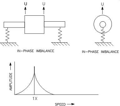
FIG. 1 Single-plane imbalance.
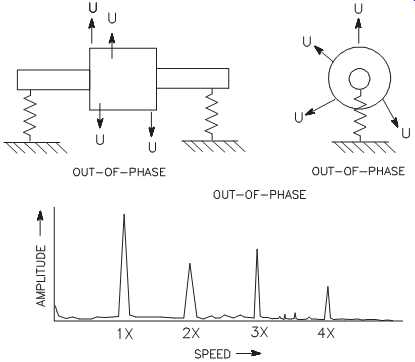
FIG. 2 Multiplane imbalance generates multiple harmonics.
Multiplane. Multiplane mechanical imbalance generates multiple harmonics of running speed. The actual number of harmonics depends on the number of imbalance points, the severity of imbalance, and the phase angle between imbalance points.
FIG. 2 illustrates a case of multiplane imbalance in which there are four out-of phase imbalance points. The resultant vibration profile contains dominant frequencies at 1x, 2x, 3x, and 4x. The actual amplitude of each of these components is determined by the amount of imbalance at each of the four points, but the 1x component should always be higher than any subsequent harmonics.
Lift/Gravity Differential:
Lift, which is designed into a machine-train's rotating elements to compensate for the effects of gravity acting on the rotor, is another source of imbalance. Because lift does not always equal gravity, some imbalance always exists in machine-trains. The vibration component caused by the lift/gravity differential effect appears at the fundamental or 1x frequency.
Other:
All failure modes create some form of imbalance in a machine, as do aerodynamic instability, hydraulic instability, and process loading. The process loading of most machine-trains varies, at least slightly, during normal operations. These vibration components appear at the 1x frequency.
Mechanical Looseness
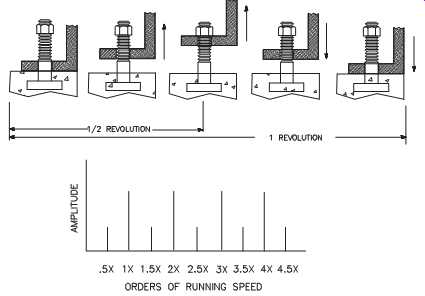
FIG. 3 Vertical mechanical looseness has a unique vibration profile.
Looseness, which can be present in both the vertical and horizontal planes, can create a variety of patterns in a vibration signature. In some cases, the fundamental (1x) frequency is excited. In others, a frequency component at one-half multiples of the shaft's running speed (e.g., 0.5x, 1.5x, 2.5x) is present. In almost all cases, there are multiple harmonics, both full and half.
Vertical:
Mechanical looseness in the vertical plane generates a series of harmonic and half harmonic frequency components. FIG. 3 is a simple example of a vertical mechanical looseness signature.
In most cases, the half-harmonic components are about one-half of the amplitude of the harmonic components. They result from the machine-train lifting until stopped by the bolts. The impact as the machine reaches the upper limit of travel generates a frequency component at one-half multiples (i.e., orders) of running speed. As the machine returns to the bottom of its movement, its original position, a larger impact occurs that generates the full harmonics of running speed.
The difference in amplitude between the full harmonics and half-harmonics is caused by the effects of gravity. As the machine lifts to its limit of travel, gravity resists the lifting force. Therefore, the impact force that is generated as the machine foot contacts the mounting bolt is the difference between the lifting force and gravity. As the machine drops, the force of gravity combines with the force generated by imbalance.
The impact force as the machine foot contacts the foundation is the sum of the force of gravity and the force resulting from imbalance.
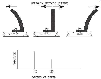
FIG. 4 Horizontal looseness creates first and second harmonics.
Horizontal:
FIG. 4 illustrates horizontal mechanical looseness, which is also common to machine-trains. In this example, the machine's support legs flex in the horizontal plane. Unlike the vertical looseness illustrated in FIG. 37, gravity is uniform at each leg and there is no increased impact energy as the leg's direction is reversed.
Horizontal mechanical looseness generates a combination of first (1x) and second (2x) harmonic vibrations. Because the energy source is the machine's rotating shaft, the timing of the flex is equal to one complete revolution of the shaft, or 1x. During this single rotation, the mounting legs flex to their maximum deflection on both sides of neutral. The double change in direction as the leg first deflects to one side then the other generates a frequency at two times (2x) the shaft's rotating speed.
Other:
Many other forms of mechanical looseness (besides vertical and horizontal movement of machine legs) are typical for manufacturing and process machinery. Most forms of pure mechanical looseness result in an increase in the vibration amplitude at the fundamental (1x) shaft speed. In addition, looseness generates one or more harmonics (i.e., 2x, 3x, 4x, or combinations of harmonics and half-harmonics); however, not all looseness generates this classic profile. For example, excessive bearing and gear clearances don’t generate multiple harmonics. In these cases, the vibration profile contains unique frequencies that indicate looseness, but the profile varies depending on the nature and severity of the problem.
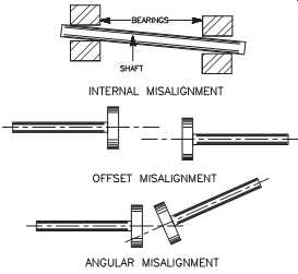
FIG. 5 Three types of misalignment.
With sleeve or Babbitt bearings, looseness is displayed as an increase in subharmonic frequencies (i.e., less than the actual shaft speed, such as 0.5x). Rolling-element bearings display elevated frequencies at one or more of their rotational frequencies. Excessive gear clearance increases the amplitude at the gear-mesh frequency and its sidebands.
Other forms of mechanical looseness increase the noise floor across the entire band width of the vibration signature. Although the signature does not contain a distinct peak or series of peaks, the overall energy contained in the vibration signature is increased. Unfortunately, the increase in noise floor cannot always be used to detect mechanical looseness. Some vibration instruments lack sufficient dynamic range to detect changes in the signature's noise floor.
Misalignment
This condition is virtually always present in machine-trains. Generally, we assume that misalignment exists between shafts that are connected by a coupling, V-belt, or other intermediate drive; however, it can also exist between bearings of a solid shaft and at other points within the machine.
How misalignment appears in the vibration signature depends on the type of mis alignment. FIG. 5 illustrates three types of misalignment (i.e., internal, offset, and angular). These three types excite the fundamental (1x) frequency component because they create an apparent imbalance condition in the machine.
Internal (i.e., bearing) and offset misalignment also excites the second (2x) harmonic frequency. The shaft creates two high spots as it turns through one complete revolution. These two high spots create the first (1x) and second harmonic (2x) components.
Angular misalignment can take several signature forms and excites the fundamental (1x) and secondary (2x) components. It can excite the third (3x) harmonic frequency depending on the actual phase relationship of the angular misalignment. It also creates a strong axial vibration.
Modulations
Modulations are frequency components that appear in a vibration signature but cannot be attributed to any specific physical cause or forcing function. Although these frequencies are "ghosts" or artificial frequencies, they can result in significant damage to a machine-train. The presence of ghosts in a vibration signature often leads to mis interpretation of the data.
Ghosts are caused when two or more frequency components couple, or merge, to form another discrete frequency component in the vibration signature. This generally occurs with multiple-speed machines or a group of single-speed machines.
Note that the presence of modulation, or ghost peaks, is not an absolute indication of a problem within the machine-train. Couple effects may simply increase the amplitude of the fundamental running speed and do little damage to the machine-train; however, this increased amplitude will amplify any defects within the machine-train.
Coupling can have an additive effect on the modulation frequencies, as well as being reflected as a differential or multiplicative effect. These concepts are discussed in the sections to follow.
Take as an example the case of a 10-tooth pinion gear turning at 10 rpm while driving a 20-tooth bullgear with an output speed of 5 rpm. This gear set generates real frequencies at 5, 10, and 100 rpm (i.e., 10 teeth x 10 rpm). This same set can also generate a series of frequencies (i.e., sum and product modulations) at 15 rpm (i.e., 10 rpm + 5 rpm) and 150 rpm (i.e., 15 rpm x 10 teeth). In this example, the 10-rpm input speed coupled with the 5-rpm output speed to create ghost frequencies driven by this artificial fundamental speed (15 rpm).
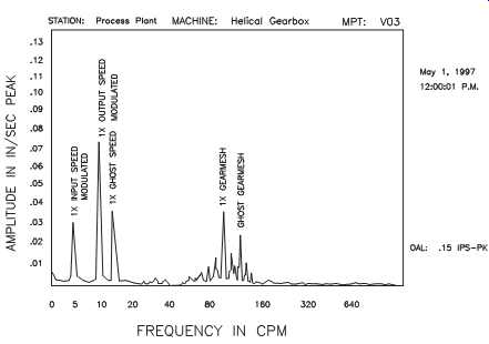
FIG. 6 Sum modulation for a speed-increaser gearbox.
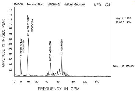
FIG. 7 Difference modulation for a speed-increaser gearbox.
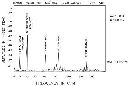
FIG. 8 Product modulation for a speed-increaser gearbox.
Sum:
This type of modulation, which is described in the previous example, generates a series of frequencies that include the fundamental shaft speeds, both input and output, and fundamental gear-mesh profile. The only difference between the real frequencies and the ghost is their location on the frequency scale. Instead of being at the actual shaft speed frequency, the ghost appears at frequencies equal to the sum of the input and output shaft speeds. FIG. 6 illustrates this for a speed-increaser gearbox.
Difference:
In this case, the resultant ghost, or modulation, frequencies are generated by the difference between two or more speeds (see FIG. 7). If we use the same example as before, the resultant ghost frequencies appear at 5 rpm (i.e., 10 rpm -5 rpm) and 50 rpm (i.e., 5 rpm x 10 teeth). Note that the 5-rpm couple frequency coincides with the real output speed of 5 rpm. This results in a dramatic increase in the amplitude of one real running-speed component and the addition of a false gear-mesh peak.
This type of coupling effect is common in single-reduction/increase gearboxes or other machine-train components where multiple running or rotational speeds are relatively close together or even integer multiples of one another. It’s more destructive than other forms of coupling in that it coincides with real vibration components and tends to amplify any defects within the machine-train.
Product:
With product modulation, the two speeds couple in a multiplicative manner to create a set of artificial frequency components (see FIG. 8). In the previous example, product modulations occur at 50 rpm (i.e., 10 rpm x 5 rpm) and 500 rpm (i.e., 50 rpm x 10 teeth).
Beware that this type of coupling may often go undetected in a normal vibration analysis. Because the ghost frequencies are relatively high compared to the expected real frequencies, they are often outside the monitored frequency range used for data acquisition and analysis.
Process Instability
Normally associated with bladed or vaned machinery such as fans and pumps, process instability creates an unbalanced condition within the machine. In most cases, it excites the fundamental (1x) and blade-pass/vane-pass frequency components. Unlike true mechanical imbalance, the blade-pass and vane-pass frequency components are broader and have more energy in the form of sideband frequencies.
In most cases, this failure mode also excites the third (3x) harmonic frequency and creates strong axial vibration. Depending on the severity of the instability and the design of the machine, process instability can also create a variety of shaft-mode shapes. In turn, this excites the 1x, 2x, and 3x radial vibration components.
Resonance
Resonance is defined as a large-amplitude vibration caused by a small periodic stimulus with the same, or nearly the same, period as the system's natural vibration.
In other words, an energy source with the same, or nearly the same, frequency as the natural frequency of a machine-train or structure will excite that natural frequency. The result is a substantial increase in the amplitude of the natural frequency component.
The key point to remember is that a very low amplitude energy source can cause massive amplitudes when its frequency coincides with the natural frequency of a machine or structure. Higher levels of input energy can cause catastrophic, near instantaneous failure of the machine or structure. Every machine-train has one or more natural frequencies. If one of these frequencies is excited by some component of the normal operation of the system, the machine structure will amplify the energy, which can cause severe damage.
An example of resonance is a tuning fork. If you activate a tuning fork by striking it sharply, the fork vibrates rapidly. As long as it’s held suspended, the vibration decays with time; however, if you place it on a desktop, the fork could potentially excite the natural frequency of the desk, which would dramatically amplify the vibration energy.
The same thing can occur if one or more of the running speeds of a machine excite the natural frequency of the machine or its support structure. Resonance is a destructive vibration and, in most cases, it will cause major damage to the machine or support structure.
Two major classifications of resonance are found in most manufacturing and process plants: static and dynamic. Both types exhibit a broad-based, high-amplitude frequency component when viewed in an FFT vibration signature. Unlike meshing or passing frequencies, the resonance frequency component does not have modulations or sidebands. Instead, resonance is displayed as a single, clearly defined peak.
As illustrated in FIG. 9, a resonance peak represents a large amount of energy.
This energy is the result of both the amplitude of the peak and the broad area under the peak. This combination of high peak amplitude and broad-based energy content is typical of most resonance problems. The damping system associated with a resonance frequency is indicated by the sharpness or width of the response curve, wn, when measured at the half-power point. RMAX is the maximum resonance and is the half-power point for a typical resonance-response curve.
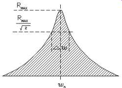
FIG. 9 Resonance response.
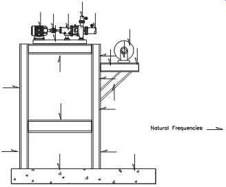
FIG. 10 Typical discrete natural frequency locations in structural
members.
Static:
When the natural frequency of a stationary, or nondynamic, structure is energized, it will resonate. This type of resonance is classified as static resonance and is considered a nondynamic phenomenon. Nondynamic structures in a machine-train include casings, bearing-support pedestals, and structural members such as beams, piping, and the like.
Because static resonance is a nondynamic phenomenon, it’s generally not associated with the primary running speed of any associated machinery. Rather, the source of static resonance can be any energy source that coincides with the natural frequency of any stationary component. For example, an I-beam support on a continuous annealing line may be energized by the running speed of a roll; however, it can also be made to resonate by a bearing frequency, overhead crane, or any of a multitude of other energy sources.
The actual resonant frequency depends on the mass, stiffness, and span of the excited member. In general terms, the natural frequency of a structural member is inversely proportional to the mass and stiffness of the member. In other words, a large turbo compressor's casing will have a lower natural frequency than that of a small end suction centrifugal pump.
FIG. 10 illustrates a typical structural-support system. The natural frequencies of all support structures, piping, and other components are functions of mass, span, and stiffness. Each of the arrows on FIG. 10 indicates a structural member or stationary machine component with a unique natural frequency. Note that each time a structural span is broken or attached to another structure, the stiffness changes. As a result, the natural frequency of that segment also changes.
Although most stationary machine components move during normal operation, they are not always resonant. Some degree of flexing or movement is common in most stationary machine-trains and structural members. The amount of movement depends on the spring constant or stiffness of the member; however, when an energy source coincides and couples with the natural frequency of a structure, excessive and extremely destructive vibration amplitudes result.
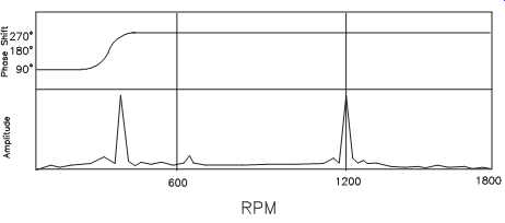
FIG. 11 Dynamic resonance phase shift.
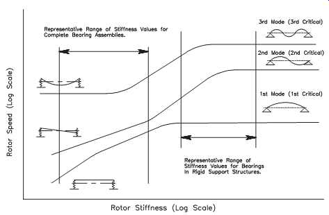
FIG. 12 Dynamic resonance plot.
Dynamic:
When the natural frequency of a rotating, or dynamic, structure (e.g., rotor assembly in a fan) is energized, the rotating element resonates. This phenomenon is classified as dynamic resonance, and the rotor speed at which it occurs is referred to as the critical.
In most cases, dynamic resonance appears at the fundamental running speed or one of the harmonics of the excited rotating element, but it can also occur at other frequencies. As in the case of static resonance, the actual natural frequencies of dynamic members depend on the mass, bearing span, shaft and bearing-support stiffness, as well as several other factors.
Confirmation Analysis. In most cases, the occurrence of dynamic resonance can be quickly confirmed. When monitoring phase and amplitude, resonance is indicated by a 180-degree phase shift as the rotor passes through the resonant zone. FIG. 11 illustrates a dynamic resonance at 500 rpm, which shows a dramatic amplitude increase in the frequency-domain display. This is confirmed by the 180-degree phase shift in the time-domain plot. Note that the peak at 1,200 rpm is not resonance. The absence of a phase shift, coupled with the apparent modulations in the FFT, discount the possibility that this peak is resonance-related.
Common Confusions. Vibration analysts often confuse resonance with other failure modes. Because many of the common failure modes tend to create abnormally high vibration levels that appear to be related to a speed change, analysts tend to miss the root-cause of these problems.
Dynamic resonance generates abnormal vibration profiles that tend to coincide with the fundamental (1x) running speed, or one or more of the harmonics, of a machine train. This often leads the analyst to incorrectly diagnose the problem as imbalance or misalignment. The major difference is that dynamic resonance is the result of a relatively small energy source, such as the fundamental running speed, that results in a massive amplification of the natural frequency of the rotating element.
Function of Speed. The high amplitudes at the rotor's natural frequency are strictly speed dependent. If the energy source, in this case speed, changes to a frequency outside the resonant zone, the abnormal vibration will disappear.
In most cases, running speed is the forcing function that excites the natural frequency of the dynamic component. As a result, rotating equipment is designed to operate at primary rotor speeds that don’t coincide with the rotor assembly's natural frequencies. Most low- to moderate-speed machines are designed to operate below the first critical speed of the rotor assembly.
Higher-speed machines may be designed to operate between the first and second, or second and third, critical speeds of the rotor assembly. As these machines accelerate through the resonant zones or critical speeds, their natural frequency is momentarily excited. As long as the ramp rate limits the duration of excitation, this mode of operation is acceptable; however, care must be taken to ensure that the transient time through the resonant zone is as short as possible.
FIG. 12 illustrates a typical critical-speed or dynamic-resonance plot. This figure is a plot of the relationship between rotor-support stiffness (X-axis) and critical rotor speed (Y-axis). Rotor-support stiffness depends on the geometry of the rotating element (i.e., shaft and rotor) and the bearing-support structure. These two dominant factors determine the response characteristics of the rotor assembly.
FAILURE MODES BY MACHINE-TRAIN COMPONENT
In addition to identifying general failure modes that are common to many types of machine-train components, failure-mode analysis can be used to identify failure modes for specific components in a machine-train; however, care must be exercised when analyzing vibration profiles because the data may reflect induced problems. Induced problems affect the performance of a specific component but are not caused by that component. For example, an abnormal outer-race passing frequency may indicate a defective rolling-element bearing. It can also indicate that abnormal loading caused by misalignment, roll bending, process instability, and so on has changed the load zone within the bearing. In the latter case, replacing the bearing does not resolve the problem, and the abnormal profile will still be present after the bearing is changed.
Bearings: Rolling Element
Bearing defects are one of the most common faults identified by vibration monitoring programs. Although bearings do wear out and fail, these defects are normally symptoms of other problems within the machine-train or process system.
Therefore, extreme care must be exercised to ensure that the real problem is identified, not just the symptom. In a rolling-element, or anti-friction, bearing vibration profile, three distinct sets of frequencies can be found: natural, rotational, and defect.
Natural Frequency:
Natural frequencies are generated by impacts of the internal parts of a rolling-element bearing. These impacts are normally the result of slight variations in load and imperfections in the machined bearing surfaces. As their name implies, these are natural frequencies and are present in a new bearing that is in perfect operating condition.
The natural frequencies of rolling-element bearings are normally well above the maximum frequency range, FMAX, used for routine machine-train monitoring.
As a result, predictive maintenance analysts rarely observe them. Generally, these frequencies are between 20KHz and 1MHz. Therefore, some vibration-monitoring programs use special high-frequency or ultrasonic monitoring techniques such as high-frequency domain (HFD). Note, however, that little is gained from monitoring natural frequencies. Even in cases of severe bearing damage, these high-frequency components add little to the analyst's ability to detect and isolate bad bearings.
Rotational Frequency:
Four normal rotational frequencies are associated with rolling-element bearings: fundamental train frequency (FTF), ball/roller spin, ball-pass outer-race, and ball-pass inner-race. The following are definitions of abbreviations that are used in the discussion to follow:
BD = Ball or roller diameter; PD = Pitch diameter; b= Contact angle (for roller = 0); n = Number of balls or rollers fr = Relative speed between the inner and outer race (rps)
Fundamental Train Frequency. The bearing cage generates the FTF as it rotates around the bearing races. The cage properly spaces the balls or rollers within the bearing races, in effect, by tying the rolling elements together and providing uniform support. Some friction exists between the rolling elements and the bearing races, even with perfect lubrication. This friction is transmitted to the cage, which causes it to rotate around the bearing races.
Because this is a friction-driven motion, the cage turns much slower than the inner race of the bearing. Generally, the rate of rotation is slightly less than one-half of the shaft speed. The FTF is calculated by the following equation:
Ball-Spin Frequency. Each of the balls or rollers within a bearing rotates around its own axis as it rolls around the bearing races. This spinning motion is referred to as ball spin, which generates a ball-spin frequency (BSF) in a vibration signature. The speed of rotation is determined by the geometry of the bearing (i.e., diameter of the ball or roller, and bearing races) and is calculated by:
Ball-Pass Outer-Race. The ball or rollers passing the outer race generate the ball-pass outer-race frequency (BPFO), which is calculated by:
Ball-Pass Inner-Race. The speed of the ball/roller rotating relative to the inner race generates the ball-pass inner-race rotational frequency (BPFI). The inner race rotates at the same speed as the shaft, and the complete set of balls/rollers passes at a slower speed. They generate a passing frequency that is determined by:
Defect Frequencies:
Rolling-element bearing defect frequencies are the same as their rotational frequencies, except for the BSF. If there is a defect on the inner race, the BPFI amplitude increases because the balls or rollers contact the defect as they rotate around the bearing. The BPFO is excited by defects in the outer race.
When one or more of the balls or rollers have a defect such as a spall (i.e., a missing chip of material), the defect impacts both the inner and outer race each time one revolution of the rolling element is made. Therefore, the defect vibration frequency is visible at two times (2x) the BSF rather than at its fundamental (1x) frequency.
Bearings: Sleeve (Babbitt)
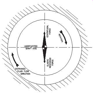
FIG. 13 A normal Babbitt bearing has balanced forces.
In normal operation, a sleeve bearing provides a uniform oil film around the supported shaft. Because the shaft is centered in the bearing, all forces generated by the rotating shaft, and all forces acting on the shaft, are equal. FIG. 13 shows the balanced forces on a normal bearing.
Lubricating-film instability is the dominant failure mode for sleeve bearings. This instability is typically caused by eccentric, or off-center, rotation of the machine shaft resulting from imbalance, misalignment, or other machine or process-related problems. FIG. 14 shows a Babbitt bearing that exhibits instability.
When oil-film instability or oil whirl occurs, frequency components at fractions (e.g., 1/4, 1/3, 3/8) of the fundamental (1x) shaft speed are excited. As the severity of the instability increases, the frequency components become more dominant in a band between 0.40 and 0.48 of the fundamental (1x) shaft speed. When the instability becomes severe enough to isolate within this band, it’s called oil whip. FIG. 15 shows the effect of increased velocity on a Babbitt bearing.
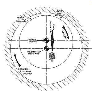
FIG. 14 Dynamics of Babbitt bearing instability.
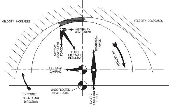
FIG. 15 Increased velocity generates an unbalanced force.
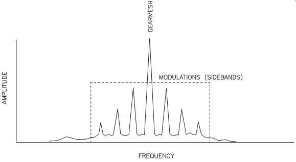
FIG. 16 Normal gear set profile is symmetrical.
Chains and Sprockets
Chain drives function in essentially the same basic manner as belt drives; however, instead of tension, chains depend on the mechanical meshing of sprocket teeth with the chain links.
Gears
All gear sets create a frequency component referred to as gear mesh. The fundamental gear-mesh frequency is equal to the number of gear teeth times the running speed of the shaft. In addition, all gear sets create a series of sidebands or modulations that are visible on both sides of the primary gear-mesh frequency.
Normal Profile:
In a normal gear set, each of the sidebands is spaced by exactly the 1x running speed of the input shaft, and the entire gear mesh is symmetrical as seen in FIG. 16.
In addition, the sidebands always occur in pairs, one below and one above the gear mesh frequency, and the amplitude of each pair is identical.
If we split the gear-mesh profile for a normal gear by drawing a vertical line through the actual mesh (i.e., number of teeth times the input shaft speed), the two halves would be identical. Therefore, any deviation from a symmetrical profile indicates a gear problem; however, care must be exercised to ensure that the problem is internal to the gears and not induced by outside influences.
External misalignment, abnormal induced loads, and a variety of other outside influences destroy the symmetry of a gear-mesh profile. For example, a single-reduction gearbox used to transmit power to a mold-oscillator system on a continuous caster drives two eccentric cams. The eccentric rotation of these two cams is transmitted directly into the gearbox, creating the appearance of eccentric meshing of the gears; however, this abnormal induced load actually destroys the spacing and amplitude of the gear-mesh profile.
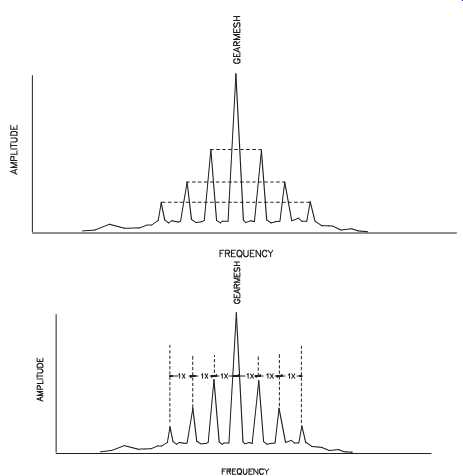
FIG. 17 Sidebands are paired and equal.
Defective Gear Profiles:
If the gear set develops problems, the amplitude of the gear-mesh frequency increases and the symmetry of the sidebands changes. The pattern illustrated in FIG. 18 is typical of a defective gear set, where overall energy is the broadband, or total, energy. Note the asymmetrical relationship of the sidebands.
Excessive Wear. FIG. 19 is the vibration profile of a worn gear set. Note that the spacing between the sidebands is erratic and is no longer evenly spaced by the input shaft speed frequency. The sidebands for a worn gear set tend to occur between the input and output speeds and are not evenly spaced.
Cracked or Broken Teeth. FIG. 20 illustrates the profile of a gear set with a broken tooth. As the gear rotates, the space left by the chipped or broken tooth increases the mechanical clearance between the pinion and bullgear. The result is a low-amplitude sideband to the left of the actual gear-mesh frequency. When the next (i.e., undamaged) teeth mesh, the added clearance results in a higher-energy impact.
The sideband to the right of the mesh frequency has much higher amplitude. As a result, the paired sidebands have nonsymmetrical amplitude, which is caused by the disproportional clearance and impact energy.
FIG. 18 Typical defective gear-mesh signature.
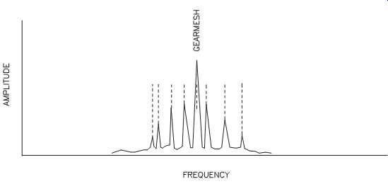
FIG. 19 Wear or excessive clearance changes the sideband spacing.
Improper Shaft Spacing:
In addition to gear-tooth wear, variations in the center-to-center distance between shafts create erratic spacing and amplitude in a vibration signature. If the shafts are too close together, the sideband spacing tends to be at input shaft speed, but the amplitude is significantly reduced. This condition causes the gears to be deeply meshed (i.e., below the normal pitch line), so the teeth maintain contact through the entire mesh. This loss of clearance results in lower amplitudes, but it exaggerates any tooth-profile defects that may be present.
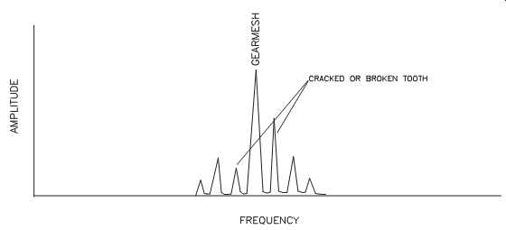
FIG. 20 A broken tooth will produce an asymmetrical sideband profile.
If the shafts are too far apart, the teeth mesh above the pitch line, which increases the clearance between teeth and amplifies the energy of the actual gear-mesh frequency and all of its sidebands. In addition, the load-bearing characteristics of the gear teeth are greatly reduced. Because the force is focused on the tip of each tooth where there is less cross-section, the stress in each tooth is greatly increased. The potential for tooth failure increases in direct proportion to the amount of excess clearance between the shafts.
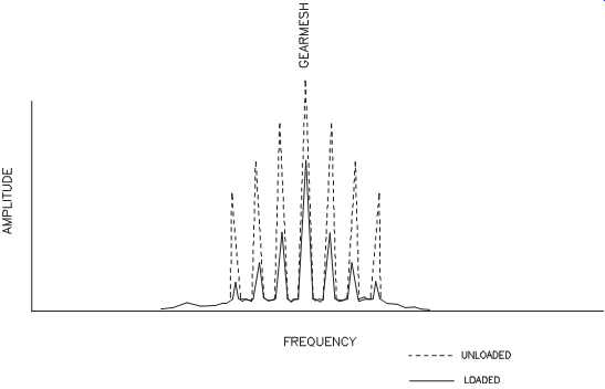
FIG. 21 Unloaded gear has much higher vibration levels.
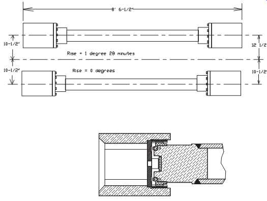
FIG. 22 Typical gear-type spindles.
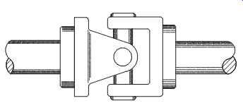
FIG. 23 Typical universal-type jackshaft.
Load Changes:
The energy and vibration profiles of gear sets change with load. When the gear is fully loaded, the profiles exhibit the amplitudes discussed previously. When the gear is unloaded, the same profiles are present, but the amplitude increases dramatically. The reason for this change is gear-tooth roughness. In normal practice, the back side of the gear tooth is not finished to the same smoothness as the power, or drive, side. Therefore, more looseness is present on the nonpower, or back, side of the gear.
FIG. 21 illustrates the relative change between a loaded and unloaded gear profile.
Jackshafts and Spindles
Another form of intermediate drive consists of a shaft with some form of universal connection on each end that directly links the prime mover to a driven unit (see FIGS. 22 and 14-23). Jackshafts and spindles are typically used in applications where the driver and driven unit are misaligned.
Most of the failure modes associated with jackshafts and spindles are the result of lubrication problems or fatigue failure resulting from overloading; however, the actual failure mode generally depends on the configuration of the flexible drive.
Lubrication Problems:
Proper lubrication is essential for all jackshafts and spindles. A critical failure point for spindles (see FIG. 22) is in the mounting pod that provides the connection between the driver and driven machine components. Mounting pods generally use either a spade-and-slipper or a splined mechanical connector. In both cases, regular application of suitable grease is essential for prolonged operation. Without proper lubrication, the mating points between the spindle's mounting pod and the machine train components impact each time the torsional power varies between the primary driver and driven component of the machine-train. The resulting mechanical damage can cause these critical drive components to fail.
In universal-type jackshafts like the one illustrated in FIG. 23, improper lubrication results in non-uniform power transmission. The absence of a uniform grease film causes the pivot points within the universal joints to bind and restrict smooth power transmission.
The typical result of poor lubrication, which results in an increase in mechanical looseness, is an increase of those vibration frequencies associated with the rotational speed.
In the case of gear-type spindles ( FIG. 22), both the fundamental (1x) and second harmonic (2x) will increase. Because the resulting forces generated by the spindle are similar to angular misalignment, the axial energy generated by the spindle will also increase significantly.
The universal-coupling configuration used by jackshafts ( FIG. 23) generates an elevated vibration frequency at the fourth (4x) harmonic of its true rotational speed.
The binding that occurs as the double pivot points move through a complete rotation causes this failure mode.
Fatigue:
Spindles and jackshafts are designed to transmit torsional power between a driver and driven unit that are not in the same plane or that have a radical variation in torsional power. Typically, both conditions are present when these flexible drives are used.
Both the jackshaft and spindle are designed to absorb transient increases or decreases in torsional power caused by twisting. In effect, the shaft or tube used in these designs winds, much like a spring, as the torsional power increases. Normally, this torque and the resultant twist of the spindle are maintained until the torsional load is reduced. At that point, the spindle unwinds, releasing the stored energy that was generated by the initial transient.
Repeated twisting of the spindle's tube or the solid shaft used in jackshafts results in a reduction in the flexible drive's stiffness. When this occurs, the drive loses some of its ability to absorb torsional transients. As a result, the driven unit may be damaged.
Unfortunately, the limits of single-channel, frequency-domain data acquisition prevent accurate measurement of this failure mode. Most of the abnormal vibration that results from fatigue occurs in the relatively brief time interval associated with startup, when radical speed changes occur, or during shutdown of the machine-train. As a result, this type of data acquisition and analysis cannot adequately capture these transients; however, the loss of stiffness caused by fatigue increases the apparent mechanical looseness observed in the steady-state, frequency-domain vibration signature. In most cases, this is similar to the mechanical looseness.
Process Rolls
Process rolls commonly encounter problems or fail because of being subjected to induced (variable) loads and from misalignment.
Induced (Variable) Loads:
Process rolls are subjected to variable loads that are induced by strip tension, tracking, and other process variables. In most cases, these loads are directional. They not only influence the vibration profile but also determine the location and orientation of data acquisition.
Strip Tension or Wrap. FIG. 24 illustrates the wrap of the strip as it passes over a series of rolls in a continuous-process line. The orientation and contact area of this wrap determines the load zone on each roll.
In this example, the strip wrap is limited to one-quarter of the roll circumference.
The load zone, or vector, on the two top rolls is on a 45-degree angle to the pass line. Therefore, the best location for the primary radial measurement is at 45 degrees opposite to the load vector. The secondary radial measurement should be 90 degrees to the primary. On the top-left roll, the secondary measurement point should be to the top left of the bearing cap; on the top-right roll, it should be at the top-right position.
The wrap on the bottom roll encompasses one-half of the roll circumferences. As a result, the load vector is directly upward, or 90 degrees, to the pass line. The best location for the primary radial-measurement point is in the vertical-downward position.
The secondary radial measurement should be taken at 90 degrees to the primary.
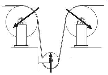
FIG. 24 Load zones determined by wrap.
Because the strip tension is slightly forward (i.e., in the direction of strip movement), the secondary measurement should be taken on the re-coiler side of the bearing cap.
Because strip tension loads the bearings in the direction of the force vector, it also tends to dampen the vibration levels in the opposite direction, or 180 degrees, of the force vector. In effect, the strip acts like a rubberband. Tension inhibits movement and vibration in the direction opposite the force vector and amplifies the movement in the direction of the force vector. Therefore, the recommended measurement-point locations provide the best representation of the roll's dynamics.
In normal operation, the force or load induced by the strip is uniform across the roll's entire face or body. As a result, the vibration profile in both the operator- and drive side bearings should be nearly identical.
Strip Width and Tracking. Strip width has a direct effect on roll loading and how the load is transmitted to the roll and its bearing-support structures. FIG. 25 illustrates a narrow strip that is tracking properly. Note that the load is concentrated on the center of the roll and is not uniform across the entire roll face.
The concentration of strip tension or load in the center of the roll tends to bend the roll. The degree of deflection depends on the following: roll diameter, roll construction, and strip tension. Regardless of these three factors, however, the vibration profile is modified. Roll bending, or deflection, increases the fundamental (1x) frequency component. The amount of increase is determined by the amount of deflection.
As long as the strip remains at the true centerline of the roll face, the vibration profile in both the operator- and drive-side bearing caps should remain nearly identical. The only exceptions are bearing rotational and defect frequencies. FIGS. 26 and 14-27 illustrate uneven loading and the resulting different vibration profiles of the operator- and drive-side bearing caps.
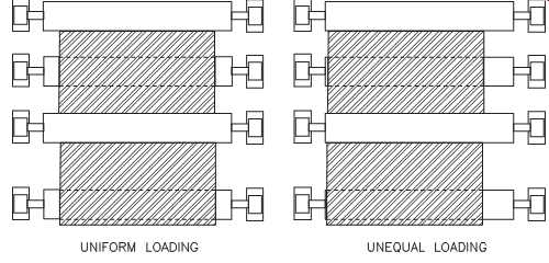
FIG. 25 Load from narrow strip concentrated in center.
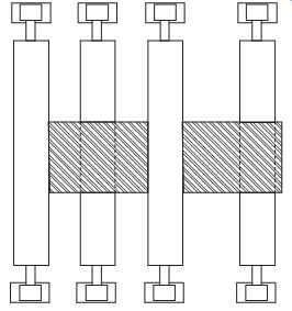
FIG. 26 Roll loading.
This extremely important factor can be used to evaluate many of the failure modes of continuous process lines. For example, the vibration profile resulting from the transmission of strip tension to the roll and its bearings can be used to determine proper roll alignment, strip tracking, and proper strip tension.
Alignment:
Process rolls must be properly aligned. The perception that they can be misaligned without causing poor quality, reduced capacity, and premature roll failure is incorrect.
In the case of single rolls (e.g., bridle and furnace rolls), they must be perpendicular to the pass line and have the same elevation on both the operator and drive sides. Roll pairs such as scrubber/backup rolls must be parallel to each other.
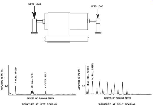
FIG. 27 Typical vibration profile with uneven loading.
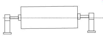
FIG. 28 Vertically misaligned roll.
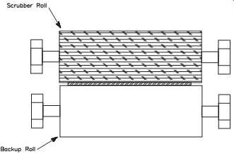
FIG. 29 Scrubber roll set.
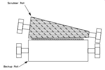
FIG. 30 Result of misalignment or nonparallel operation on brush rolls.
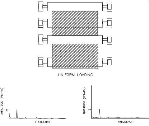
FIG. 31 Rolls in series.
Single Rolls. With the exception of steering rolls, all single rolls in a continuous process line must be perpendicular to the pass line and have the same elevation on both the operator and drive sides. Any horizontal or vertical misalignment influences the tracking of the strip and the vibration profile of the roll.
FIG. 28 illustrates a roll that does not have the same elevation on both sides (i.e., vertical misalignment). With this type of misalignment, the strip has greater tension on the side of the roll with the higher elevation, which forces it to move toward the lower end. In effect, the roll becomes a steering roll, forcing the strip to one side of the centerline.
The vibration profile of a vertically misaligned roll is not uniform. Because the strip tension is greater on the high side of the roll, the vibration profile on the high-side bearing has lower broadband energy. This is the result of damping caused by the strip tension. Dominant frequencies in this vibration profile are roll speed (1x) and outer-race defects. The low end of the roll has higher broadband vibration energy, and dominant frequencies include roll speed (1x) and multiple harmonics (i.e., the same as mechanical looseness).
Paired Rolls. Rolls that are designed to work in pairs (e.g., damming or scrubber rolls) also must be perpendicular to the pass line. In addition, they must be parallel to each other. FIG. 29 illustrates a paired set of scrubber rolls. The strip is captured between the two rolls, and the counter-rotating brush roll cleans the strip surface.
Because of the designs of both the damming and scrubber roll sets, it’s difficult to keep the rolls parallel. Most of these roll sets use a single pivot point to fix one end of the roll and a pneumatic cylinder to set the opposite end.
Other designs use two cylinders, one attached to each end of the roll. In these designs, the two cylinders are not mechanically linked and, therefore, the rolls don’t maintain their parallel relationship. The result of nonparallel operation of these paired rolls is evident in roll life.
For example, the scrubber/backup roll set should provide extended service life; however, in actual practice, the brush rolls have a service life of only a few weeks.
After this short time in use, the brush rolls will have a conical shape, much like a bottle brush (see FIG. 30). This wear pattern is visual confirmation that the brush roll and its mating rubber-coated backup roll are not parallel.
Vibration profiles can be used to determine if the roll pairs are parallel and, in this instance, the rules for parallel misalignment apply. If the rolls are misaligned, the vibration signatures exhibit a pronounced fundamental (1x) and second harmonic (2x) of roll speed.
Multiple Pairs of Rolls. Because the strip transmits the vibration profile associated with roll misalignment, it’s difficult to isolate misalignment for a continuous-process line by evaluating one single or two paired rolls. The only way to isolate such mis-alignment is to analyze a series of rolls rather than individual (or a single pair of ) rolls. This approach is consistent with good diagnostic practices and provides the means to isolate misaligned rolls and to verify strip tracking.
Strip tracking. FIG. 31 illustrates two sets of rolls in series. The bottom set of rolls is properly aligned and has good strip tracking. In this case, the vibration profiles acquired from the operator- and drive-side bearing caps are nearly identical.
Unless there is a damaged bearing, all of the profiles contain low-level roll frequencies (1x) and bearing rotational frequencies.
The top roll set is also properly aligned, but the strip tracks to the bottom of the roll face. In this case, the vibration profile from all of the bottom bearing caps contain much lower-level broadband energy, and the top bearing caps have clear indications of mechanical looseness (i.e., multiple harmonics of rotating speed). The key to this type of analysis is the comparison of multiple rolls in the order that the strip connects them.
This requires comparison of both top and bottom rolls in the order of strip pass. With proper tracking, all bearing caps should be nearly identical. If the strip tracks to one side of the roll face, all bearing caps on that side of the line will have similar profiles, but they will have radically different profiles compared to those on the opposite side.
Roll misalignment. Roll misalignment can be detected and isolated using this same method. A misaligned roll in the series being evaluated causes a change in the strip track at the offending roll. The vibration profiles of rolls upstream of the misaligned roll will be identical on both the operator and drive sides of the rolls; however, the profiles from the bearings of the misaligned roll will show a change. In most cases, they will show traditional misalignment (i.e., 1x and 2x components) but will also indicate a change in the uniform loading of the roll face. In other words, the overall or broadband vibration levels will be greater on one side than the other. The lower readings will be on the side with the higher strip tension, and the higher readings will be on the side with less tension.
The rolls following the misalignment also show a change in vibration pattern. Because the misaligned roll acts as a steering roll, the loading patterns on the subsequent rolls show different vibration levels when the operator and drive sides are compared. If the strip track was normal before the misaligned roll, the subsequent rolls will indicate off-center tracking. In those cases where the strip was already tracking off-center, a misaligned roll either improves or amplifies the tracking problem. If the misaligned roll forces the strip toward the centerline, tracking improves and the vibration profiles are more uniform on both sides. If the misaligned roll forces the strip farther off-center, the nonuniform vibration profiles will become even less uniform.
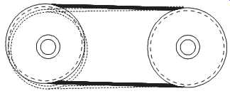
FIG. 34 Eccentric sheaves.
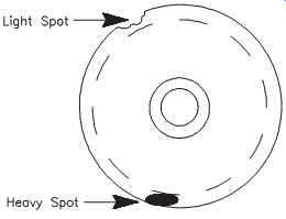
FIG. 35 Light and heavy spots on an unbalanced sheave.
Shaft
A bent shaft creates an imbalance or a misaligned condition within a machine-train.
Normally, this condition excites the fundamental (1x) and secondary (2x) running speed components in the signature; however, it’s difficult to determine the difference between a bent shaft, misalignment, and imbalance without a visual inspection.
FIGS. 32 and 14-33 illustrate the normal types of bent shafts and the force profiles that result.
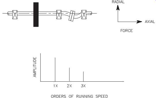
FIG. 32 Bends that change shaft length generate axial thrust.
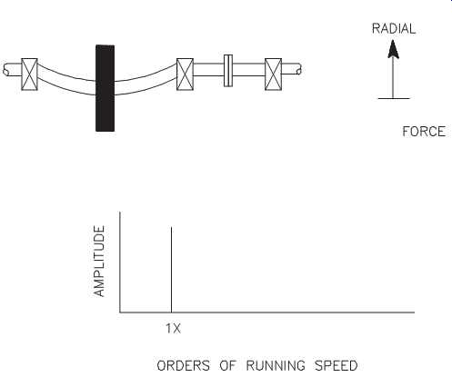
FIG. 33 Bends that don’t change shaft length generate radial forces
only.
V-Belts
V-belt drives generate a series of dynamic forces, and vibrations result from these forces. Frequency components of such a drive can be attributed to belts and sheaves.
The elastic nature of belts can either amplify or damp vibrations that are generated by the attached machine-train components.
Sheaves:
Even new sheaves are not perfect and may be the source of abnormal forces and vibration. The primary sources of induced vibration resulting from sheaves are eccentricity, imbalance, misalignment, and wear.
Eccentricity. Vibration caused by sheave eccentricity manifests itself as changes in load and rotational speed. As an eccentric drive sheave passes through its normal rotation, variations in the pitch diameter cause variations in the linear belt speed. An eccentric driven sheave causes variations in load to the drive. The rate at which such variations occur helps determine which is eccentric. An eccentric sheave may also appear to be unbalanced; however, performing a balancing operation won’t correct the eccentricity.
Imbalance. Sheave imbalance may be caused by several factors, one of which may be that it was never balanced to begin with. The easiest problem to detect is an actual imbalance of the sheave itself. A less obvious cause of imbalance is damage that has resulted in loss of sheave material. Imbalance caused by material loss can be determined easily by visual inspection, either by removing the equipment from service or by using a strobe light while the equipment is running. FIG. 35 illustrates light and heavy spots that result in sheave imbalance.
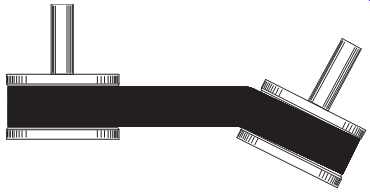
FIG. 36 Angular sheave misalignment.
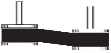
FIG. 37 Parallel sheave misalignment.
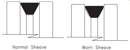
FIG. 38 Normal and worn sheave grooves.

FIG. 39 Typical spectral plot (i.e., vibration profile) of a defective
belt.
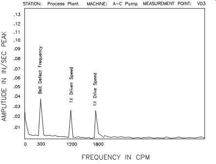
FIG. 40 Spectral plot of shaft rotational and belt defect (i.e., imbalance)
frequencies.
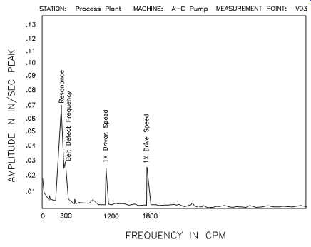
FIG. 41 Spectral plot of resonance excited by belt-defect frequency.
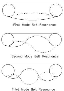
FIG. 42 Examples of mode resonance in a belt span.
Misalignment. Sheave misalignment most often produces axial vibration at the shaft rotational frequency (1x) and radial vibration at one and two times the shaft rotational frequency (1x and 2x). This vibration profile is similar to coupling misalignment.
FIG. 36 illustrates angular sheave misalignment, and FIG. 37 illustrates parallel misalignment.
Wear. Worn sheaves may also increase vibration at certain rotational frequencies; however, sheave wear is more often indicated by increased slippage and drive wear.
FIG. 38 illustrates both normal and worn sheave grooves.
Belts:
V-belt drives typically consist of multiple belts mated with sheaves to form a means of transmitting motive power. Individual belts, or an entire set of belts, can generate abnormal dynamic forces and vibration. The dominant sources of belt-induced vibrations are defects, imbalance, resonance, tension, and wear.
Defects. Belt defects appear in the vibration signature as subsynchronous peaks, often with harmonics. FIG. 39 shows a typical spectral plot (i.e., vibration profile) for a defective belt.
Imbalance. An imbalanced belt produces vibration at its rotational frequency. If a belt's performance is initially acceptable and later develops an imbalance, the belt has most likely lost material and must be replaced. If imbalance occurs with a new belt, it’s defective and must be replaced. FIG. 40 shows a spectral plot of shaft rotational and belt defect (i.e., imbalance) frequencies.
Resonance. Belt resonance occurs primarily when the natural frequency of some length of the belt is excited by a frequency generated by the drive. Occasionally, a sheave may also be excited by some drive frequency. FIG. 41 shows a spectral plot of resonance excited by belt-defect frequency.
Adjusting the span length, belt thickness, and belt tension can control belt resonance.
Altering any of these parameters changes the resonance characteristics. In most applications, it’s not practical to alter the shaft rotational speeds, which are also possible sources of the excitation frequency.
Resonant belts are readily observable visually as excessive deflection, or belt whip. It can occur in any resonant mode, so there may or may not be inflection points observed along the span. FIG. 42 illustrates first-, second-, and third-mode resonance in a belt span.
Tension. Loose belts can increase the vibration of the drive, often in the axial plane.
In the case of multiple V-belt drives, mismatched belts also aggravate this condition.
Improper sheave alignment can also compromise tension in multiple-belt drives.
Wear. Worn belts slip, and the primary indication is speed change. If the speed of the driver increases and the speed of the driven unit decreases, then slippage is probably occurring. This condition may be accompanied by noise and smoke, causing belts to overheat and be glazed in appearance. It’s important to replace worn belts.