| HOME | Project Management Data Warehousing / Mining Software Testing | Technical Writing |
|
3. EFFORT ESTIMATION One of the crucial aspects of project planning and management is understanding how much the project is likely to cost. Cost overruns can cause customers to cancel projects, and cost underestimates can force a project team to invest much of its time without financial compensation. As described in SIDEBAR 3, there are many reasons for inaccurate estimates. A good cost estimate early in the project's life helps the project manager to know how many developers will be required and to arrange for the appropriate staff to be available when they are needed. The project budget pays for several types of costs: facilities, staff, methods, and tools. The facilities costs include hardware, space, furniture, telephones, modems, heating and air conditioning, cables, disks, paper, pens, photocopiers, and all other items that provide the physical environment in which the developers will work. For some projects, this environment may already exist, so the costs are well -understood and easy to estimate. But for other projects, the environment may have to be created. For example, a new project may require a security vault, a raised floor, temperature or humidity controls or special furniture. Here, the costs can be estimated, but they may vary from initial estimates as the environment is built or changed. For instance, installing cabling in a building may seem straightforward until the builders discover that the building is of special historical significance, so that the cables must be routed around the walls instead of through them. =========== SIDEBAR 3 CAUSES OF INACCURATE ESTIMATES Lederer and Prasad (1992) investigated the cost -estimation practices of 115 different organizations. Thirty-five percent of the managers surveyed on a five-point Likert scale indicated that their current estimates were "moderately unsatisfactory" or "very unsatisfactory." The key causes identified by the respondents included:
Several aspects of the project were noted as key influences on the estimate:
===========
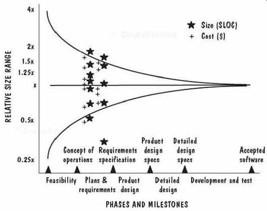
There are sometimes hidden costs that are not apparent to the managers and developers. For example, studies indicate that a programmer needs a minimum amount of space and quiet to be able to work effectively. McCue (1978) reported to his colleagues at IBM that the minimum standard for programmer work space should be 100 square feet of dedicated floor space with 30 square feet of horizontal work surface. The space also needs a floor -to -ceiling enclosure for noise protection. DeMarco and Lister's (1987) work suggests that programmers free from telephone calls and uninvited visitors are more efficient and produce a better product than those who are subject to repeated interruption. Other project costs involve purchasing software and tools to support development efforts. In addition to tools for designing and coding the system, the project may buy software to capture requirements, organize documentation, test the code, keep track of changes, generate test data, support group meetings, and more. These tools, sometimes called Computer-Aided Software Engineering (or CASE) tools, are some times required by the customer or are part of a company's standard software development process. The two types of organizational structure can be combined, where appropriate. For instance, programmers may be asked to develop a subsystem on their own, using an egoless approach within a hierarchical structure. Or the test team of a loosely structured project may impose a hierarchical structure on itself and designate one person to be responsible for all major testing decisions. For most projects, the biggest component of cost is effort. We must determine how many staff-days of effort will be required to complete the project. Effort is certainly the cost component with the greatest degree of uncertainty. We have seen how work style, project organization, ability, interest, experience, training, and other employee characteristics can affect the time it takes to complete a task. Moreover, when a group of workers must communicate and consult with one another, the effort needed is increased by the time required for meetings, documentation, and training. Cost, schedule, and effort estimation must be done as early as possible during the project's life cycle, since it affects resource allocation and project feasibility. (If it costs too much, the customer may cancel the project.) But estimation should be done repeatedly throughout the life cycle; as aspects of the project change, the estimate can be refined, based on more complete information about the project's characteristics. FIG. 12 illustrates how uncertainty early in the project can affect the accuracy of cost and size estimates (Boehm et al. 1995). The stars represent size estimates from actual projects, and the pluses are cost estimates. The funnel-shaped lines narrowing to the right represent Boehm's sense of how our estimates get more accurate as we learn more about a project. Notice that when the specifics of the project are not yet known, the estimate can differ from the eventual actual cost by a factor of 4. As decisions are made about the product and the process, the factor decreases. Many experts aim for estimates that are within 10 percent of the actual value, but Boehm's data indicate that such estimates typically occur only when the project is almost done-too late to be useful for project management. To address the need for producing accurate estimates, software engineers have developed techniques for capturing the relationships among effort and staff characteristics, project requirements, and other factors that can affect the time, effort, and cost of developing a software system. For the rest of this section, we focus on effort-estimation techniques. Expert Judgment Many effort-estimation methods rely on expert judgment. Some are informal techniques, based on a manager's experience with similar projects. Thus, the accuracy of the prediction is based on the competence, experience, objectivity, and perception of the estimator. In its simplest form, such an estimate makes an educated guess about the effort needed to build an entire system or its subsystems. The complete estimate can be computed from either a top -down or a bottom -up analysis of what is needed. Many times analogies are used to estimate effort. If we have already built a system much like the one proposed, then we can use the similarity as the basis for our estimates. For example, if system A is similar to system B, then the cost to produce system A should be very much like the cost to produce B. We can extend the analogy to say that if A is about half the size or complexity of B, then A should cost about half as much as B. The analogy process can be formalized by asking several experts to make three predictions: a pessimistic one (x), an optimistic one (z), and a most likely guess (y). Then our estimate is the mean of the beta probability distribution determined by these numbers: (x + 4y + z)/6. By using this technique, we produce an estimate that "normalizes" the individual estimates. The Delphi technique makes use of expert judgment in a different way. Experts are asked to make individual predictions secretly, based on their expertise and using whatever process they choose. Then, the average estimate is calculated and presented to the group. Each expert has the opportunity to revise his or her estimate, if desired. The process is repeated until no expert wants to revise. Some users of the Delphi technique discuss the average before new estimates are made; at other times, the users allow no discussion. And in another variation, the justifications of each expert are circulated anonymously among the experts. Wolverton (1974) built one of the first models of software development effort. His software cost matrix captures his experience with project cost at TRW, a U.S. soft ware development company. As shown in TABLE 6, the row name represents the type of software, and the column designates its difficulty. Difficulty depends on two factors: whether the problem is old (O) or new (N) and whether it is easy (E), moderate (M), or hard (H). The matrix elements are the cost per line of code, as calibrated from historical data at TRW. To use the matrix, you partition the proposed software system into modules. Then, you estimate the size of each module in terms of lines of code. Using the matrix, you calculate the cost per module, and then sum over all the modules. For instance, suppose you have a system with three modules: one input/output module that is old and easy, one algorithm module that is new and hard, and one data management module that is old and moderate. If the modules are likely to have 100, 200, and 100 lines of code, respectively, then the Wolverton model estimates the cost to be (100 X 17) + (200 X 35) + (100 X 31) = $11,800. TABLE 6 Wolverton Model Cost Matrix Since the model is based on TRW data and uses 1974 dollars, it is not applicable to today's software development projects. But the technique is useful and can be trans ported easily to your own development or maintenance environment. In general, experiential models, by relying mostly on expert judgment, are subject to all its inaccuracies. They rely on the expert's ability to determine which projects are similar and in what ways. However, projects that appear to be very similar can in fact be quite different. For example, fast runners today can run a mile in 4 minutes. A marathon race requires a runner to run 26 miles and 365 yards. If we extrapolate the 4-minute time, we might expect a runner to run a marathon in 1 hour and 45 minutes. Yet a marathon has never been run in under 2 hours. Consequently, there must be characteristics of running a marathon that are very different from those of running a mile. Like wise, there are often characteristics of one project that make it very different from another project, but the characteristics are not always apparent. Even when we know how one project differs from another, we do not always know how the differences affect the cost. A proportional strategy is unreliable, because project costs are not always linear: Two people cannot produce code twice as fast as one. Extra time may be needed for communication and coordination, or to accommodate differences in interest, ability, and experience. Sackman, Erikson, and Grant (1968) found that the productivity ratio between best and worst programmers averaged 10 to 1, with no easily definable relationship between experience and performance. Likewise, a more recent study by Hughes (1996) found great variety in the way software is designed and developed, so a model that may work in one organization may not apply to another. Hughes also noted that past experience and knowledge of available resources are major factors in determining cost. Expert judgment suffers not only from variability and subjectivity, but also from dependence on current data. The data on which an expert judgment model is based must reflect current practices, so they must be updated often. Moreover, most expert judgment techniques are simplistic, neglecting to incorporate a large number of factors that can affect the effort needed on a project. For this reason, practitioners and researchers have turned to algorithmic methods to estimate effort. Algorithmic Methods Researchers have created models that express the relationship between effort and the factors that influence it. The models are usually described using equations, where effort is the dependent variable, and several factors (such as experience, size, and application type) are the independent variables. Most of these models acknowledge that project size is the most influential factor in the equation by expressing effort as: E = (a + bSc)m(X) where S is the estimated size of the system, and a, b, and c are constants. X is a vector of cost factors, x1 through xn, and m is an adjustment multiplier based on these factors. In other words, the effort is determined mostly by the size of the proposed system, adjusted by the effects of several other project, process, product, or resource characteristics. =========== TABLE 7 Walston and Felix Model Productivity Factors 1. Customer interface complexity 2. User participation in requirements definition 3. Customer -originated program design changes 4. Customer experience with the application area 5. Overall personnel experience 6. Percentage of development programmers who participated in the design of functional specifications 7. Previous experience with the operational computer 8. Previous experience with the programming language 9. Previous experience with applications of similar size and complexity 10. Ratio of average staff size to project duration (people per month) 11. Hardware under concurrent development 12. Access to development computer open under special request 13. Access to development computer closed 14. Classified security environment for computer and at least 25% of programs and data 15. Use of structured programming 16. Use of design and code inspections 17. Use of top -down development 18. Use of a chief programmer team 19. Overall complexity of code 20. Complexity of application processing 21. Complexity of program flow 22. Overall constraints on program's design 23. Design constraints on the program's main storage 24. Design constraints on the program's timing 25. Code for real-time or interactive operation A or for execution under severe time constraints 26. Percentage of code for delivery 27. Code classified as nonmathematical application and input/output formatting programs 28. Number of classes of items in the database per 1000 lines of code 29. Number of pages of delivered documentation per 1000 lines of code ========== TABLE 8 Bailey-Basili Effort Modifiers =========== Each of the 29 factors was weighted by 1 if the factor increases productivity, 0 if it has no effect on productivity, and -1 if it decreases productivity. A weighted sum of the 29 factors was then used to generate an effort estimate from the basic equation. Bailey and Bashi (1981) suggested a modeling technique, called a meta-model, for building an estimation equation that reflects your own organization's characteristics. They demonstrated their technique using a database of 18 scientific projects written in Fortran at NASA's Goddard Space Flight Center. First, they minimized the standard error estimate and produced an equation that was very accurate: E=ss+n 71V-16 Then, they adjusted this initial estimate based on the ratio of errors. If R is the ratio between the actual effort, E, and the predicted effort, E', then the effort adjustment is defined as JR - 1 E Rad/ - 1/R if R 1 if R < 1 They then adjusted the initial effort estimate E_adj this way: {(1 ERadi)E E ad; = E/(1 + ERadj) if R 1 if R < 1 Finally, Bailey and Basil (1981) accounted for other factors that affect effort, shown in TABLE 8. For each entry in the table, the project is scored from 0 (not present) to 5 (very important), depending on the judgment of the project manager. Thus, the total score for METH can be as high as 45, for CPLX as high as 35, and for EXP as high as 25. Their model describes a procedure, based on multi-linear least -square regression, for using these scores to further modify the effort estimate. Clearly, one of the problems with models of this type is their dependence on size as a key variable. Estimates are usually required early, well before accurate size information is available, and certainly before the system is expressed as lines of code. So the models simply translate the effort -estimation problem to a size -estimation problem. Boehm's Constructive Cost Model (COCOMO) acknowledges this problem and incorporates three sizing techniques in the latest version, COCOMO II. Boehm (1981) developed the original COCOMO model in the 1970s, using an extensive database of information from projects at TRW, an American company that built software for many different clients. Considering software development from both an engineering and an economics viewpoint, Boehm used size as the primary determinant of cost and then adjusted the initial estimate using over a dozen cost drivers, including attributes of the staff, the project, the product, and the development environment. In the 1990s, Boehm updated the original COCOMO model, creating COCOMO II to reflect the ways in which software development had matured. The COCOMO II estimation process reflects three major stages of any development project. Whereas the original COCOMO model used delivered source lines of code as its key input, the new model acknowledges that lines of code are impossible to know early in the development cycle. At stage 1, projects usually build prototypes to resolve high -risk issues involving user interfaces, software and system interaction, performance, or technological maturity. Here, little is known about the likely size of the final product under consideration, so COCOMO II estimates size in what its creators call application points. As we shall see, this technique captures size in terms of high level effort generators, such as the number of screens and reports, and the number of third-generation language components. At stage 2, the early design stage, a decision has been made to move forward with development, but the designers must explore alternative architectures and concepts of operation. Again, there is not enough information to support fine-grained effort and duration estimation, but far more is known than at stage 1. For stage 2, COCOMO II employs function points as a size measure. Function points, a technique explored in depth in IFPUG (1994a and b), estimate the functionality captured in the requirements, so they offer a richer system description than application points. By stage 3, the post-architecture stage, development has begun, and far more information is known. In this stage, sizing can be done in terms of function points or lines of code, and many cost factors can be estimated with some degree of comfort. COCOMO II also includes models of reuse, takes into account maintenance and breakage (i.e., the change in requirements over time), and more. As with the original COCOMO, the model includes cost factors to adjust the initial effort estimate. A research group at the University of Southern California is assessing and improving its accuracy. Let us look at COCOMO II in more detail. The basic model is of the form E = b m(X) where the initial size -based estimate, bSc, is adjusted by the vector of cost driver information, m(X). TABLE 9 describes the cost drivers at each stage, as well as the use of other models to modify the estimate. TABLE 9 Three Stages of COCOMO II At stage 1, application points supply the size measure. This size measure is an extension of the object -point approach suggested by Kauffman and Kumar (1993) and productivity data reported by Banker, Kauffman, and Kumar (1992). To compute application points, you first count the number of screens, reports, and third -generation language components that will be involved in the application. It is assumed that these elements are defined in a standard way as part of an integrated computer -aided soft ware engineering environment. Next, you classify each application element as simple, medium, or difficult. TABLE 10 contains guidelines for this classification. TABLE 10 Application Point Complexity Levels of reuse, requirements change, and maintenance. The scale (i.e., the value for c in the effort equation) had been set to 1.0 in stage 1; for stage 2, the scale ranges from 0.91 to The number to be used for simple, medium, or difficult application points is a complexity weight found in TABLE 11. The weights reflect the relative effort required to implement a report or screen of that complexity level. Then, you sum the weighted reports and screens to obtain a single application-point number. If r percent of the objects will be reused from previous projects, the number of new application points is calculated to be: New application points = (application points) x (100 - r )/100 To use this number for effort estimation, you use an adjustment factor, called a productivity rate, based on developer experience and capability, coupled with CASE maturity and capability. For example, if the developer experience and capability are rated low, and the CASE maturity and capability are rated low, then TABLE 12 tells us that the productivity factor is 7, so the number of person -months required is the number of new application points divided by 7. When the developers' experience is low but CASE maturity is high, the productivity estimate is the mean of the two values: 16. Likewise, when a team of developers has experience levels that vary, the productivity estimate can use the mean of the experience and capability weights. TABLE 11 Complexity Weights for Application Points TABLE 12 Productivity Estimate Calculation At stage 1, the cost drivers are not applied to this effort estimate. However, at stage 2, the effort estimate, based on a function -point calculation, is adjusted for degree 1.23, depending on the degree of novelty of the system, conformity, early architecture and risk resolution, team cohesion, and process maturity. The cost drivers in stages 2 and 3 are adjustment factors expressed as effort multi pliers based on rating your project from "extra low" to "extra high," depending on its characteristics. For example, a development team's experience with an application type is considered to be:
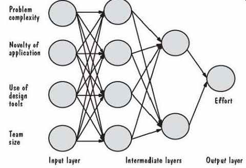
Similarly, analyst capability is measured on an ordinal scale based on percentile ranges. For instance, the rating is "very high" if the analyst is in the ninetieth percentile and "nominal" for the fifty-fifth percentile. Correspondingly, COCOMO II assigns an effort multiplier ranging from 1.42 for very low to 0.71 for very high. These multipliers reflect the notion that an analyst with very low capability expends 1.42 times as much effort as a nominal or average analyst, while one with very high capability needs about three quarters the effort of an average analyst. Similarly, TABLE 13 lists the cost driver categories for tool use, and the multipliers range from 1.17 for very low to 0.78 for very high. ======== TABLE 13 Tool Use Categories Category Meaning Very low Edit, code, debug Low Simple front-end, back -end CASE, little integration Nominal Basic life -cycle tools, moderately integrated High Strong, mature life -cycle tools, moderately integrated Very high Strong, mature, proactive life -cycle tools, well -integrated with processes, methods, reuse ========= Notice that stage 2 of COCOMO II is intended for use during the early stages of design. The set of cost drivers in this stage is smaller than the set used in stage 3, reflecting lesser understanding of the project's parameters at stage 2. The various components of the COCOMO model are intended to be tailored to fit the characteristics of your own organization. Tools are available that implement COCOMO II and compute the estimates from the project characteristics that you sup ply. Later in this section, we will apply COCOMO to our information system example. Machine-Learning Methods In the past, most effort- and cost-modeling techniques have relied on algorithmic methods. That is, researchers have examined data from past projects and generated equations from them that are used to predict effort and cost on future projects. How ever, some researchers are looking to machine learning for assistance in producing good estimates. For example, neural networks can represent a number of interconnected, interdependent units, so they are a promising tool for representing the various activities involved in producing a software product. In a neural network, each unit (called a neuron and represented by network node) represents an activity; each activity has inputs and outputs. Each unit of the network has associated software that performs an accounting of its inputs, computing a weighted sum; if the sum exceeds a threshold value, the unit produces an output. The output, in turn, becomes input to other related units in the net work, until a final output value is produced by the network. The neural network is, in a sense, an extension or the activity graphs we examined earlier in this section. There are many ways for a neural network to produce its outputs. Some techniques involve looking back to what has happened at other nodes; these are called back-propagation techniques. They are similar to the method we used with activity graphs to look back and determine the slack on a path. Other techniques look forward, to anticipate what is about to happen. Neural networks are developed by "training" them with data from past projects. Relevant data are supplied to the network, and the network uses forward and back ward algorithms to "learn" by identifying patterns in the data. For example, historical data about past projects might contain information about developer experience; the network may identify relationships between level of experience and the amount of effort required to complete a project. FIG. 13 illustrates how Shepperd (1997) used a neural network to produce an effort estimate. There are three layers in the network, and the network has no cycles. The four inputs are factors that can affect effort on a project; the network uses them to produce effort as the single output. To begin, the network is initialized with random weights. Then, new weights, calculated as a "training set" of inputs and outputs based on past history, are fed to the network. The user of the model specifies a training algorithm that explains how the training data are to be used; this algorithm is also based on past history, and it commonly involves back -propagation. Once the network is trained (i.e., once the network values are adjusted to reflect past experience), it can then be used to estimate effort on new projects.
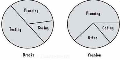
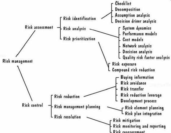
Several researchers have used back -propagation algorithms on similar neural networks to predict development effort, including estimation for projects using fourth -generation languages (Wittig and Finnie 1994; Srinivasan and Fisher 1995; Samson, Ellison, and Dugard 1997). Shepperd (1997) reports that the accuracy of this type of model seems to be sensitive to decisions about the topology of the neural network, the number of learning stages, and the initial random weights of the neurons within the network. The networks also seem to require large training sets in order to give good predictions. In other words, they must be based on a great deal of experience rather than a few representative projects. Data of this type are sometimes difficult to obtain, especially collected consistently and in large quantity, so the paucity of data limits this technique's usefulness. Moreover, users tend to have difficulty understanding neural networks. However, if the technique produces more accurate estimates, organizations may be more willing to collect data for the networks. In general, this "learning" approach has been tried in different ways by other researchers. Srinivasan and Fisher (1995) used Kemerer's data (Kemerer 1989) with a statistical technique called a regression tree; they produced predictions more accurate than those of the original COCOMO model and SLIM, a proprietary commercial model. However, their results were not as good as those produced by a neural network or a model based on function points. Briand, Basili, and Thomas (1992) obtained better results from using a tree induction technique, using the Kemerer and COCOMO datasets. Porter and Selby (1990) also used a tree-based approach; they constructed a decision tree that identifies which project, process, and product characteristics may be useful in predicting likely effort. They also used the technique to predict which modules are likely to be fault-prone. A machine -learning technique called Case -Based Reasoning (CBR) can be applied to analogy -based estimates. Used by the artificial intelligence community, CBR builds a decision algorithm based on the several combinations of inputs that might be encountered on a project. Like the other techniques described here, CBR requires information about past projects. Shepperd (1997) points out that CBR offers two clear advantages over many of the other techniques. First, CBR deals only with events that actually occur, rather than with the much larger set of all possible occurrences. This same feature also allows CBR to deal with poorly understood domains. Second, it is easier for users to understand particular cases than to depict events as chains of rules or as neural networks. Estimation using CBR involves four steps: 1. The user identifies a new problem as a case. 2. The system retrieves similar cases from a repository of historical information. 3. The system reuses knowledge from previous cases. 4. The system suggests a solution for the new case. The solution may be revised, depending on actual events, and the outcome is placed in the repository, building up the collection of completed cases. However, there are two big hurdles in creating a successful CBR system: characterizing cases and determining similarity. Cases are characterized based on the information that happens to be available. Usually, experts are asked to supply a list of features that are significant in describing cases and, in particular, in determining when two cases are similar. In practice, similarity is usually measured using an n -dimensional vector of n features. Shepperd, Schofield, and Kitchenham (1996) found a CBR approach to be more accurate than traditional regression analysis -based algorithmic methods. Finding the Model for Your Situation There are many effort and cost models being used today: commercial tools based on past experience or intricate models of development, and home-grown tools that access databases of historical information about past projects. Validating these models (i.e., making sure the models reflect actual practice) is difficult, because a large amount of data is needed for the validation exercise. Moreover, if a model is to apply to a large and varied set of situations, the supporting database must include measures from a very large and varied set of development environments. Even when you find models that are designed for your development environment, you must be able to evaluate which are the most accurate on your projects. There are two statistics that are often used to help you in assessing the accuracy, PRED and MMRE. PRED(x/100) is the percentage of projects for which the estimate is within x% of the actual value. For most effort, cost, and schedule models, managers evaluate PRED(0.25), that is, those models whose estimates are within 25% of the actual value; a model is considered to function well if PRED(0.25) is greater than 75%. MMRE is the mean magnitude of relative error, so we hope that the MMRE for a particular model is very small. Some researchers consider an MMRE of 0.25 to be fairly good, and Boehm (1981) suggests that MMRE should be 0.10 or less. TABLE 14 lists the best values for PRED and MMRE reported in the literature for a variety of models. As you can see, the statistics for most models are disappointing, indicating that no model appears to have captured the essential characteristics and their relationships for all types of development. However, the relationships among cost factors are not simple, and the models must be flexible enough to handle changing use of tools and methods. TABLE 14 Summary of Model Performance Moreover, Kitchenham, MacDonell, Pickard, and Shepperd (2000) point out that the MMRE and PRED statistics are not direct measures of estimation accuracy. They suggest that you use the simple ratio of estimate to actual: estimate/actual. This mea sure has a distribution that directly reflects estimation accuracy. By contrast, MMRE and PRED are measures of the spread (standard deviation) and peakedness (kurtosis) of the ratio, so they tell us only characteristics of the distribution. Even when estimation models produce reasonably accurate estimates, we must be able to understand which types of effort are needed during development. For example, designers may not be needed until the requirements analysts have finished developing the specification. Some effort and cost models use formulas based on past experience to apportion the effort across the software development life cycle. For instance, the original COCOMO model suggested effort required by development activity, based on percentages allotted to key process activities. But, as FIG. 14 illustrates, researchers report conflicting values for these percentages (Brooks 1995; Yourdon 1982). Thus, when you are building your own database to support estimation in your organization, it is important to record not only how much effort is expended on a project, but also who is doing it and for what activity. ========== SIDEBAR 4 BOEHM'S TOP TEN RISK ITEMS Boehm (19911 identities 10 risk items and recommends risk management techniques to 15 address them. 1. Personnel shortfalls. Staffing with top talent; job matching; team building; morale building; cross -training; pre-scheduling key people. 2. Unrealistic schedules and budgets. Detailed multisource cost and schedule estimation; design to cost; incremental development; software reuse; requirements scrubbing. 3. Developing the wrong software functions. Organizational analysis; mission analysis; operational concept formulation; user surveys; prototyping; early user's manuals. 4. Developing the wrong user interface. Prototyping; scenarios; task analysis. 5. Gold plating. Requirements scrubbing; prototyping; cost -benefit analysis; design to cost. 6. Continuing stream of requirements changes. High change threshold; information hiding; incremental development (defer changes to later increments). 7. Shortfalls in externally performed tasks. Reference checking; pre-award audits; award -fee contracts; competitive design or prototyping; team building. 8. Shortfalls in externally furnished components. Benchmarking; inspections; reference checking; compatibility analysis. 9. Real-time performance shortfalls. Simulation; benchmarking; modeling; prototyping; instrumentation; tuning. 10. Straining computer science capabilities Technical analysis; cost -benefit analysis; prototyping; reference checking. =========== 4. RISK MANAGEMENT As we have seen, many software project managers take steps to ensure that their projects are done on time and within effort and cost constraints. However, project management involves far more than tracking effort and schedule. Managers must determine whether any unwelcome events may occur during development or maintenance and make plans to avoid these events or, if they are inevitable, minimize their negative consequences. A risk is an unwanted event that has negative consequences. Project managers must engage in risk management to understand and control the risks on their projects. What Is a Risk? Many events occur during software development; SIDEBAR 4 lists Boehm's view of some of the riskiest one& We distinguish risks from other project events by looking for three things (Rook 1993): 1. A loss associated with the event. The event must create a situation where some thing negative happens to the project: a loss of time, quality, money, control, understanding, and so on. For example, if requirements change dramatically after the design is done, then the project can suffer from loss of control and under standing if the new requirements are for functions or features with which the design team is unfamiliar. And a radical change in requirements is likely to lead to losses of time and money if the design is not flexible enough to be changed quickly and easily. The loss associated with a risk is called the risk impact. 2. The likelihood that the event will occur. We must have some idea of the probability that the event will occur. For example, suppose a project is being developed on one machine and will be ported to another when the system is fully tested. If the second machine is a new model to be delivered by the vendor, we must estimate the likelihood that it will not be ready on time. The likelihood of the risk, measured from 0 (impossible) to 1 (certainty) is called the risk probability. When the risk probability is 1, then the risk is called a problem, since it is certain to happen. 3. The degree to which we can change the outcome. For each risk, we must determine what we can do to minimize or avoid the impact of the event. Risk control involves a set of actions taken to reduce or eliminate a risk. For example, if the requirements may change after design, we can minimize the impact of the change by creating a flexible design. If the second machine is not ready when the software is tested, we may be able to identify other models or brands that have the same functionality and performance and can run our new software until the new model is delivered. We can quantify the effects of the risks we identify by multiplying the risk impact by the risk probability, to yield the risk exposure. For example, if the likelihood that the requirements will change after design is 0.3, and the cost to redesign to new requirements is $50,000, then the risk exposure is $15,000. Clearly, the risk probability can change over time, as can the impact, so part of a project manager's job is to track these values over time and plan for the events accordingly. There are two major sources of risk: generic risks and project -specific risks. Generic risks are those common to all software projects, such as misunderstanding the requirements, losing key personnel, or allowing insufficient time for testing. Project-specific risks are threats that result from the particular vulnerabilities of the given project. For example, a vendor may be promising network software by a particular date, but there is some risk that the network software will not be ready on time. Risk Management Activities Risk management involves several important steps, each of which is illustrated in FIG. 15. First, we assess the risks on a project, so that we understand what may occur during the course of development or maintenance. The assessment consists of three activities: identifying the risks, analyzing them, and assigning priorities to each of them. To identify them, we may use many different techniques.
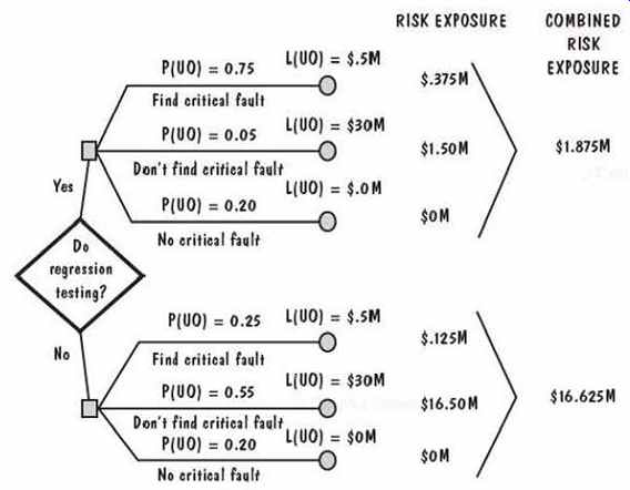
If the system we are building is similar in some way to a system we have built before, we may have a checklist of problems that may occur; we can review the check list to determine if the new project is likely to be subject to the risks listed. For systems that are new in some way, we may augment the checklist with an analysis of each of the activities in the development cycle; by decomposing the process into small pieces, we may be able to anticipate problems that may arise. For example, we may decide that there is a risk of the chief designer leaving during the design process. Similarly, we may analyze the assumptions or decisions we make about how the project will be done, who will do it, and with what resources. Then, each assumption is assessed to determine the risks involved. Finally, we analyze the risks we have identified, so that we can understand as much as possible about when, why, and where they might occur. There are many techniques we can use to enhance our understanding, including system dynamics models, cost models, performance models, network analysis, and more. Once we have itemized all the risks, we use our understanding to assign priorities them. A priority scheme enables us to devote our limited resources only to the most threatening risks. Usually, priorities are based on the risk exposure, which takes into account not only likely impact, but also the probability of occurrence. The risk exposure is computed from the risk impact and the risk probability, so we must estimate each of these risk aspects. To see how the quantification is done, consider the analysis depicted in FIG. 16. Suppose we have analyzed the system development process and we know we are working under tight deadlines for delivery. We have decided to build the system in a series of releases, where each release has more functionality than the one that preceded it. Because the system is designed so that functions are relatively independent, we consider testing only the new functions for a release, and we assume that the existing functions still work as they did before. However, we may worry that there are risks associated with not performing regression testing the assurance that existing functionality still works correctly.
For each possible outcome, we estimate two quantities: the probability of an unwanted outcome, P(UO), and the loss associated with the unwanted outcome, P(UO), and the loss associated with the unwanted outcome, L(UO). For instance, there are three possible consequences of performing regression testing: finding a critical fault if one exists, not finding the critical fault (even though it exists), or deciding (correctly) that there is no critical fault. As the figure illustrates, we have estimated the probability of the first case to be 0.75, of the second to be 0.05, and of the third to be 0.20. The loss associated with an unwanted outcome is estimated to be $500,000 if a critical fault is found, so that the risk exposure is $375,000. Similarly, we calculate the risk exposure for the other branches of this decision tree, and we find that our risk exposure if we perform regression testing is almost $2 million. However, the same kind of analysis shows us that the risk exposure if we do not perform regression testing is almost $17 million. Thus, we say (loosely) that more is at risk if we do not perform regression testing. Risk exposure helps us to list the risks in priority order, with the risks of most concern given the highest priority. Next, we must take steps to control the risks. The notion of control acknowledges that we may not be able to eliminate all risk& Instead, we may be able to minimize the risk or mitigate it by taking action to handle the unwanted out come in an acceptable way. Therefore, risk control involves risk reduction, risk planning, and risk resolution. There are three strategies for risk reduction:
To aid decision making about risk reduction, we must take into account the cost of reducing the risk. We call risk leverage the difference in risk exposure divided by the cost of reducing the risk. In other words, risk reduction leverage is: (Risk exposure before reduction - risk exposure after reduction) / (cost of risk reduction) If the leverage value is not high enough to justify the action, then we can look for other less costly or more effective reduction techniques. In some cases, we can choose a development process to help reduce the risk. For example, we saw in Section 2 that prototyping can improve understanding of the requirements and design, so selecting a prototyping process can reduce many project risks. It is useful to record decisions in a risk management plan, so that both customer and development team can review how problems are to be avoided, as well as how they are to be handled should they arise. Then, we should monitor the project as development progresses, periodically reevaluating the risks, their probability, and their likely impact. 5. THE PROJECT PLAN To communicate risk analysis and management, project cost estimates, schedule, and organization to our customers, we usually write a document called a project plan. The plan puts in writing the customer's needs, as well as what we hope to do to meet them. The customer can refer to the plan for information about activities in the development process, making it easy to follow the project's progress during development. We can also use the plan to confirm with the customer any assumptions we are making, especially about cost and schedule. A good project plan includes the following items: 1. project scope 2. project schedule 3. project team organization 4. technical description of the proposed system 5. project standards, procedures, and proposed techniques and tools 6. quality assurance plan 7. configuration management plan 8. documentation plan 9. data management plan 10. resource management plan 11. test plan 12. training plan 13. security plan 14. risk management plan 15. maintenance plan The scope defines the system boundary, explaining what will be included in the system and what will not be included. It assures the customer that we understand what is wanted. The schedule can be expressed using a work breakdown structure, the deliverables, and a timeline to show what will be happening at each point during the project life cycle. A Gantt chart can be useful in illustrating the parallel nature of some of the development tasks. The project plan also lists the people on the development team, how they are organized, and what they will be doing. As we have seen, not everyone is needed all the time during the project, so the plan usually contains a resource allocation chart to show staffing, levels at different times. Writing a technical description forces us to answer questions and address issues as we anticipate how development will proceed. This description lists hardware and software, including compilers, interfaces, and special-purpose equipment or software. Any special restrictions on cabling, execution time, response time, security, or other aspects of functionality or performance are documented in the plan. The plan also lists any standards or methods that must be used, such as:
For large projects, it may be appropriate to include a separate quality assurance plan, to describe how reviews, inspections, testing, and other techniques will help to evaluate quality and ensure that it meets the customer's needs. Similarly, large projects need a configuration management plan, especially when there are to be multiple versions and releases of the system. As we will see in Section 10, configuration management helps to control multiple copies of the software. The configuration management plan tells the customer how we will track changes to the requirements, design, code, test plans, and documents. Many documents are produced during development, especially for large projects where information about the design must be made available to project team members. the project plan lists the documents that will be produced, explains who will write them and when, and, in concert with the configuration management plan, describes how documents will be changed. Because every software system involves data for input, calculation, and output, the project plan must explain how data will be gathered, stored, manipulated, and archived. The plan should also explain how resources will be used. For example, if the hardware configuration includes removable disks, then the resource management part of the project plan should explain what data are on each disk and how the disk packs or diskettes will be allocated and backed up. Testing requires a great deal of planning to be effective, and the project plan describes the project's overall approach to testing. In particular, the plan should state how test data will be generated, how each program module will be tested (e.g., by testing all paths or all statements), how program modules will be integrated with each other and tested, how the entire system will be tested, and who will perform each type of testing. Sometimes, systems are produced in stages or phases, and the test plan should explain how each stage will be tested. When new functionality is added to a sys tem in stages, as we saw in Section 2, then the test plan must address regression testing, ensuring that the existing functionality still works correctly. Training classes and documents are usually prepared during development, rather than after the system is complete, so that training can begin as soon as the system is ready ( and sometimes before). The project plan explains how training will occur, describing each class, supporting software and documents, and the expertise needed by each student. When a system has security requirements, a separate security plan is sometimes needed. The security plan addresses the way that the system will protect data, users, and hardware. Since security involves confidentiality, availability, and integrity, the plan must explain how each facet of security affects system development. For example, if access to the system will be limited by using passwords, then the plan must describe who issues and maintains the passwords, who develops the password -handling soft ware, and what the password encryption scheme will be. Finally, if the project team will maintain the system after it is delivered to the user, the project plan should discuss responsibilities for changing the code, repairing the hardware, and updating supporting documentation and training materials. |