AMAZON multi-meters discounts AMAZON oscilloscope discounts
AMAZON multi-meters discounts
AMAZON oscilloscope discounts
.
.This section discusses normal failure modes, monitoring techniques that
can prevent premature failures, and the measurement points required for monitoring
common machine-train components. Understanding the specific location and orientation
of each measurement point is critical to diagnosing incipient problems.
The frequency-domain, or FFT, signature acquired at each measurement point is an actual representation of the individual machine-train component's motion at that point on the machine. Without knowing the specific location and orientation, it’s difficult- if not impossible-to correctly identify incipient problems. In simple terms, the FFT signature is a photograph of the mechanical motion of a machine-train in a specific direction and at a specific point and time.
The vibration-monitoring process requires a large quantity of data to be collected, temporarily stored, and downloaded to a more powerful computer for permanent storage and analysis. In addition, there are many aspects to collecting meaningful data. Data collection generally is accomplished using microprocessor-based data collection equipment referred to as vibration analyzers; however, before analyzers can be used, it’s necessary to set up a database with the data collection and analysis parameters.
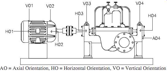
FIG. 1 Recommended measurement point logic. AO = Axial Orientation,
HO = Horizontal Orientation, VO = Vertical Orientation
The term narrowband refers to a specific frequency window that is monitored because of the knowledge that potential problems may occur as a result of known machine components or characteristics in this frequency range.
The orientation of each measurement point is an important consideration during the database setup and analysis. Each measurement point on every machine-train in a predictive maintenance program has an optimum orientation. For example, a helical gear set creates specific force vectors during normal operation. As the gear set degrades, these force vectors transmit the maximum vibration components. If only one radial reading is acquired for each bearing housing, it should be oriented in the plane that provides the greatest vibration amplitude.
For continuity, each machine-train should be set up on a "common-shaft" with the outboard driver bearing designated as the first data point. Measurement points should be numbered sequentially, starting with the outboard driver bearing and ending with the outboard bearing of the final driven component. This point is illustrated in FIG. 1. Any numbering convention may be used, but it should be consistent, which pro vides two benefits:
1. Immediate identification of the location of a particular data point during the analysis/diagnostic phase.
2. Grouping the data points by "common shaft" enables the analyst to evaluate all parameters affecting each component of a machine-train.
DRIVERS
All machines require some form of motive power, which is referred to as a driver.
This section includes the monitoring parameters for the two most common drivers: electric motors and steam turbines.
Electric Motors
Electric motors are the most common source of motive power for machine-trains. As a result, more of them are evaluated using microprocessor-based vibration-monitoring systems than any other driver. The vibration frequencies of the following parameters are monitored to evaluate operating condition. This information is used to establish a database.
- Bearing frequencies
- Imbalance
- Line frequency
- Loose rotor bars
- Running speed
- Slip frequency
- V-belt intermediate drives
Bearing Frequencies
Electric motors may incorporate either sleeve or rolling-element bearings. A narrow band window should be established to monitor both the normal rotational and defect frequencies associated with the type of bearing used for each application.
Imbalance
Electric motors are susceptible to a variety of forcing functions that cause instability or imbalance. The narrowbands established to monitor the fundamental and other harmonics of actual running speed are useful in identifying mechanical imbalance, but other indices should also be used.
One such index is line frequency, which provides indications of instability. Modulations, or harmonics, of line frequency may indicate the motor's inability to find and hold magnetic center. Variations in line frequency also increase the amplitude of the fundamental and other harmonics of running speed.
Axial movement and the resulting presence of a third harmonic of running speed is another indication of instability or imbalance within the motor. The third harmonic is present whenever axial thrusting of a rotating element occurs.
Line Frequency
Many electrical problems-or problems associated with the quality of the incoming power and internal to the motor-can be isolated by monitoring the line frequency. Line frequency refers to the frequency of the alternating current being sup plied to the motor. In the case of 60-cycle power, the fundamental or first harmonic (60Hz), second harmonic (120Hz), and third harmonic (180Hz) should be monitored.
Loose Rotor Bars
Loose rotor bars are a common failure mode of electric motors. Two methods can be used to identify them. The first method uses high-frequency vibration components that result from oscillating rotor bars. Typically, these frequencies are well above the normal maximum frequency used to establish the broadband signature. If this is the case, a high-pass filter such as high-frequency domain can be used to monitor the condition of the rotor bars.
The second method uses the slip frequency to monitor for loose rotor bars. The passing frequency created by this failure mode energizes modulations associated with slip.
This method is preferred because these frequency components are within the normal bandwidth used for vibration analysis.
Running Speed
The running speed of electric motors, both alternating current (AC) and direct current (DC), varies. Therefore, for monitoring purposes, these motors should be classified as variable-speed machines. A narrowband window should be established to track the true running speed.
Slip Frequency
Slip frequency is the difference between synchronous speed and actual running speed of the motor. A narrowband filter should be established to monitor electrical line frequency. The window should have enough resolution to clearly identify the frequency and the modulations, or sidebands that represent slip frequency.
Normally, these modulations are spaced at the difference between synchronous and actual speed, and the number of sidebands is equal to the number of poles in the motor.
V-Belt Intermediate Drives
Electric motors with V-belt intermediate drive display the same failure modes as those described previously; however, the unique V-belt frequencies should be monitored to determine if improper belt tension or misalignment is evident.
In addition, electric motors used with V-belt intermediate drive assemblies are susceptible to premature wear on the bearings. Typically, electric motors are not designed to compensate for the sideloads associated with V-belt drives. In this type of application, special attention should be paid to monitoring motor bearings.
The primary data-measurement point on the inboard bearing housing should be located in the plane opposing the induced load (side-load), with the secondary point at 90 degrees. The outboard primary data-measurement point should be in a plane opposite the inboard bearing, with the secondary at 90 degrees.
Steam Turbines
There are wide variations in the size of steam turbines, which range from large utility units to small package units designed as drivers for pumps, and so on. The following section describes in general terms the monitoring guidelines. Parameters that should be monitored are bearings, blade pass, mode shape (shaft deflection), and speed (both running and critical).
Bearings:
Turbines use both rolling-element and Babbitt bearings. Narrowbands should be established to monitor both the normal rotational frequencies and failure modes of the specific bearings used in each turbine.
Blade Pass:
Turbine rotors consist of a series of vanes or blades mounted on individual wheels.
Each of the wheel units, which are referred to as a stage of compression, has a different number of blades. Narrowbands should be established to monitor the blade-pass frequency of each wheel. Loss of a blade or flexing of blades or wheels is detected by these narrowbands.
Mode Shape (Shaft Deflection):
Most turbines have relatively long bearing spans and highly flexible shafts. These factors, coupled with variations in process flow conditions, make turbine rotors highly susceptible to shaft deflection during normal operation. Typically, turbines operate in either the second or third mode and should have narrowbands at the second (2X) and third (3X) harmonics of shaft speed to monitor for mode shape.
Speed:
All turbines are variable-speed drivers and operate near or above one of the rotor's critical speeds. Narrowbands should be established that track each of the critical speeds defined for the turbine's rotor. In most applications, steam turbines operate above the first critical speed and in some cases above the second. A movable narrowband window should be established to track the fundamental (1X), second (2X), and third (3X) harmonics of actual shaft speed. The best method is to use orders analysis and a tachometer to adjust the window location.
Normally, the critical speeds are determined by the mechanical design and should not change; however, changes in the rotor configuration or a buildup of calcium or other foreign materials on the rotor will affect them. The narrowbands should be wide enough to permit some increase or decrease.
INTERMEDIATE DRIVES
Intermediate drives transmit power from the primary driver to a driven unit or units.
Included in this classification are chains, couplings, gearboxes, and V-belts.
Chains
In terms of its vibration characteristics, a chain-drive assembly is much like a gear set. The meshing of the sprocket teeth and chain links generates a vibration profile that is almost identical to that of a gear set. The major difference between these two machine-train components is that the looseness or slack in the chain tends to modulate and amplify the tooth-mesh energy. Most of the forcing functions generated by a chain-drive assembly can be attributed to the forces generated by tooth-mesh. The typical frequencies associated with chain-drive assembly monitoring are those of running speed, tooth-mesh, and chain speed.
Running Speed:
Chain-drives normally are used to provide positive power transmission between a driver and driven unit where direct coupling cannot be accomplished. Chain-drives generally have two distinct running speeds: driver or input speed and driven or output speed. Each of the shaft speeds is clearly visible in the vibration profile, and a discrete narrowband window should be established to monitor each of the running speeds.
These speeds can be calculated using the ratio of the drive to driven sprocket. For example, where the drive sprocket has a circumference of 10 inches and the driven sprocket a circumference of 5 inches, the output speed will be two times the input speed. Tooth-mesh narrowband windows should be created for both the drive and driven tooth-meshing frequencies. The windows should be broad enough to capture the sidebands or modulations that this type of passing frequency generates. The frequency of the sprocket-teeth meshing with the chain links, or passing frequency, is calculated by the following formula:
Tooth - Mesh Frequency = Number of Sprocket Teeth ¥ Shaft Speed
Unlike gear sets, a chain-drive system can have two distinctive tooth-mesh frequencies. Because the drive and driven sprockets don’t directly mesh, the meshing frequency generated by each sprocket is visible in the vibration profile.
Chain Speed:
The chain acts much like a driven gear and has a speed that is unique to its length.
The chain speed is calculated by the following equation:
Chain Speed = 25 teeth 1 rpm 250 links cpm rpm ¥
== =
For example:
00 2500 250 10 10 Chain Speed =
Number of Drive Sprocket Teeth, Shaft Speed, Number of Links in Chain
Couplings
Couplings cannot be monitored directly, but they generate forcing functions that affect the vibration profile of both the driver and driven machine-train component. Each coupling should be evaluated to determine the specific mechanical forces and failure modes they generate. This section discusses flexible couplings, gear couplings, jack shafts, and universal joints.
Flexible Couplings:
Most flexible couplings use an elastomer or spring-steel device to provide power trans mission from the driver to the driven unit. Both coupling types create unique mechanical forces that directly affect the dynamics and vibration profile of the machine-train.
The most obvious force with flexible couplings is endplay or movement in the axial plane. Both the elastomer and spring-steel devices have memory, which forces the axial position of both the drive and driven shafts to a neutral position. Because of their flexibility, these devices cause the shaft to move constantly in the axial plane. This is exhibited as harmonics of shaft speed. In most cases, the resultant profile is a signature that contains the fundamental (1X) frequency and second (2X) and third (3X) harmonics.
Gear Couplings:
When properly installed and maintained, gear-type couplings don’t generate a unique forcing function or vibration profile; however, excessive wear, variations in speed or torque, or over-lubrication results in a forcing function.
Excessive wear or speed variation generates a gear-mesh profile that corresponds to the number of teeth in the gear coupling multiplied by the rotational speed of the driver. Because these couplings use a mating gear to provide power transmission, variations in speed or excessive clearance permit excitation of the gear-mesh profile.
Jackshafts:
Some machine-trains use an extended or spacer shaft, called a jackshaft, to connect the driver and a driven unit. This type of shaft may use any combination of flexible coupling, universal joint, or splined coupling to provide the flexibility required to make the connection. Typically, this type of intermediate drive is used either to absorb torsional variations during speed changes or to accommodate misalignment between the two machine-train components.
Because of the length of these shafts and the flexible couplings or joints used to transmit torsional power, jackshafts tend to flex during normal operation. Flexing results in a unique vibration profile that defines its operating mode shape.
In relatively low-speed applications, the shaft tends to operate in the first mode or with a bow between the two joints. This mode of operation generates an elevated vibration frequency at the fundamental (1X) turning speed of the jackshaft. In higher speed applications, or where the flexibility of the jackshaft increases, it deflects into an "S" shape between the two joints. This "S" or second-mode shape generates an elevated frequency at both the fundamental (1X) frequency and the second harmonic (2X) of turning speed. In extreme cases, the jackshaft de?ects further and operates in the third mode. When this happens, it generates distinct frequencies at the fundamental (1X), second harmonic (2X), and third harmonic (3X) of turning speed.
As a rule, narrowband windows should be established to monitor at least these three distinct frequencies (i.e., 1X, 2X, and 3X). In addition, narrowbands should be estab lished to monitor the discrete frequencies generated by the couplings or joints used to connect the jackshaft to the driver and driven unit.
Universal Joints:
A variety of universal joints is used to transmit torsional power. In most cases, this type of intermediate drive is used when some misalignment between the drive and driven unit is necessary. Because of the misalignment, the universal's pivot points gen erate a unique forcing function that in?uences both the dynamics and vibration pro?le generated by a machine-train.
Figure 2 illustrates a typical double-pivot universal joint. This type of joint, which is similar to those used in automobiles, generates a unique frequency at four times (4X) the rotational speed of the shaft. Each of the pivot-point bearings generates a passing frequency each time the shaft completes a revolution.
Gearboxes
Gear sets are used to change speed or rotating direction of the primary driver. The basic monitoring parameters for all gearboxes include bearings, gear-mesh frequen cies, and running speeds.
Bearings:
Avariety of bearing types is used in gearboxes. Narrowband windows should be estab lished to monitor the rotational and defect frequencies generated by the speci?c type of bearing used in each application.
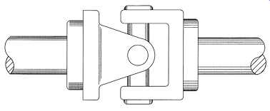
FIG. 2 Typical double-pivot universal joint.
Special attention should be given to the thrust bearings, which are used in conjunction with helical gears. Because helical gears generate a relatively strong axial force, each gear shaft must have a thrust bearing located on the backside of the gear to absorb the thrust load. Therefore, all helical gear sets should be monitored for shaft run-out.
The thrust, or positioning, bearing of a herringbone or double-helical gear has little or no normal axial loading; however, a coupling lockup can cause severe damage to the thrust bearing. Double-helical gears usually have only one thrust bearing, typically on the bullgear. Therefore, the thrust-bearing rotor should be monitored with at least one axial data-measurement point.
The gear mesh should be in a plane opposing the preload, creating the primary data measurement point on each shaft. A secondary data-measurement point should be located at 90 degrees to the primary point.
Gear-Mesh Frequencies:
Each gear set generates a unique profile of frequency components that should be monitored. The fundamental gear-mesh frequency is equal to the number of teeth in the pinion or drive gear multiplied by the rotational shaft speed. In addition, each gear set generates a series of modulations, or sidebands, that surround the fundamental gear mesh frequency. In a normal gear set, these modulations are spaced at the same frequency as the rotational shaft speed and appear on both sides of the fundamental gear mesh.
A narrowband window should be established to monitor the fundamental gear-mesh profile. The lower and upper limits of the narrowband should include the modulations generated by the gear set. The number of sidebands will vary depending on the resolution used to acquire data. In most cases, the narrowband limits should be about 10 percent above and below the fundamental gear-mesh frequency.
A second narrowband window should be established to monitor the second harmonic (2X) of gear mesh. Gear misalignment and abnormal meshing of gear sets result in multiple harmonics of the fundamental gear-mesh profile. This second window provides the ability to detect potential alignment or wear problems in the gear set.
Running Speeds:
A narrowband window should be established to monitor each of the running speeds generated by the gear sets within the gearbox. The actual number of running speeds varies depending on the number of gear sets. For example, a single-reduction gearbox has two speeds: input and output. A double-reduction gearbox has three speeds: input, intermediate, and output. Intermediate and output speeds are determined by calculations based on input speed and the ratio of each gear set. FIG. 3 illustrates a typical double-reduction gearbox.
If the input speed is 1,800 rotations per minute (rpm), then the intermediate and output speeds are calculated using the following:
Output Speed:
Intermediate Speed Number of Intermediate Gear Teeth Number of Output Gear Teeth
Intermediate Speed Input Speed Number of Input Gear Teeth Number of Intermediate Gear Teeth
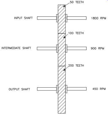
FIG. 3 Double-reduction gearbox.
===
Table 1 Belt-Drive Failure: Symptoms, Causes, and Corrective Actions
Symptom Cause Corrective Action High 1X rotational frequency in Unbalanced or eccentric Balance or replace sheave.
radial direction. sheave.
High 1X belt frequency with Defects in belt. Replace belt.
harmonics. Impacting at belt frequency in waveform.
High 1X belt frequency. Unbalanced belt. Replace belt.
Sinusoidal waveform with period of belt frequency.
High 1X rotational frequency in Loose, misaligned, or Align sheaves, re-tension or axial plane. 1X and possibly 2X mismatched belts. replace belts as needed. radial.
Source: Integrated Systems, Inc.
===
V-Belts:
V-belts are common intermediate drives for fans, blowers, and other types of machinery. Unlike some other power-transmission mechanisms, V-belts generate unique forcing functions that must be understood and evaluated as part of a vibration analysis. The key monitoring parameters for V-belt-driven machinery are fault frequency and running speed.
Most of the forcing functions generated by V-belt drives can be attributed to the elastic or rubberband effect of the belt material. This elasticity is needed to pro vide the traction required to transmit power from the drive sheave (i.e., pulley) to the driven sheave. Elasticity causes belts to act like springs, increasing vibration in the direction of belt wrap, but damping it in the opposite direction. As a result, belt elasticity tends to accelerate wear and the failure rate of both the driver and driven unit.
Fault Frequencies:
Belt-drive fault frequencies are the frequencies of the driver, the driven unit, and the belt. In particular, frequencies at one times the respective shaft speeds indicate faults with the balance, concentricity, and alignment of the sheaves. The belt frequency and its harmonics indicate problems with the belt. Table 1 summarizes the symptoms and causes of belt-drive failures, as well as corrective actions.
Running Speeds:
Belt-drive ratios may be calculated if the pitch diameters (see FIG. 5) of the sheaves are known. This coefficient, which is used to determine the driven speed given the drive speed, is obtained by dividing the pitch diameter of the drive sheave by the pitch diameter of the driven sheave. These relationships are expressed by the following equations:
Drive Speed, rpm Driven Speed, rpm Driven Sheave Diameter Drive Sheave Diameter
Drive Reduction Drive Sheave Diameter Driven Sheave Diameter
Using these relationships, the sheave rotational speeds can be determined; however, obtaining the other component speeds requires a bit more effort. The rotational speed of the belt cannot directly be determined using the information presented so far. To Using these relationships, the sheave rotational speeds can be determined; however, obtaining the other component speeds requires a bit more effort. The rotational speed of the belt cannot directly be determined using the information presented so far. To calculate belt rotational speed (rpm), the linear belt speed must first be determined by finding the linear speed (in./min.) of the sheave at its pitch diameter. In other words, multiply the pitch circumference (PC) by the rotational speed of the sheave, where:
Pitch Circumference in Pitch Diameter in Linear Speed in min Pitch Circumference in Sheave Speed rpm () =¥ () () = () ¥ () p
To find the exact rotational speed of the belt (rpm), divide the linear speed by the length of the belt:
Belt Rotational Speed rpm Linear Speed in min Belt Length in () =() ()
To approximate the rotational speed of the belt, the linear speed may be calculated using the pitch diameters and the center-to-center distance (see FIG. 4) between the sheaves. This method is accurate only if there is no belt sag. Otherwise, the belt rotational speed obtained using this method is slightly higher than the actual value.
In the special case where the drive and driven sheaves have the same diameter, the formula for determining the belt length is as follows:
The following equation is used to approximate the belt length where the sheaves have different diameters:
Belt Length Drive PC Driven PC 2 Center Distance = + +¥ () 2
Center Distance
Belt Length = Pitch Circumference + (2 ¥ Center Distance)
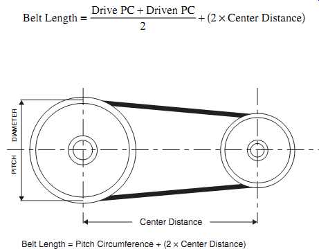
FIG. 4 Pitch diameter and center-to-center distance between belt sheaves.
DRIVEN COMPONENTS
This module cannot effectively discuss all possible combinations of driven components that may be found in a plant; however, the guidelines provided in this section can be used to evaluate most of the machine-trains and process systems that are typically included in a microprocessor-based vibration-monitoring program.
Compressors:
There are two basic types of compressors: centrifugal and positive displacement. Both of these major classifications can be further divided into subtypes, depending on their operating characteristics. This section provides an overview of the more common centrifugal and positive-displacement compressors.
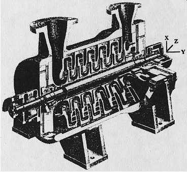
FIG. 5 Typical inline centrifugal compressor.
Centrifugal:
There are two types of commonly used centrifugal compressors: inline and bullgear.
Inline. The inline centrifugal compressor functions in exactly the same manner as a centrifugal pump. The only difference between the pump and the compressor is that the compressor has smaller clearances between the rotor and casing. Therefore, inline centrifugal compressors should be monitored and evaluated in the same manner as centrifugal pumps and fans. As with these driven components, the inline centrifugal compressor consists of a single shaft with one or more impeller(s) mounted on the shaft. All components generate simple rotating forces that can be monitored and evaluated with ease. FIG. 5 shows a typical inline centrifugal compressor.
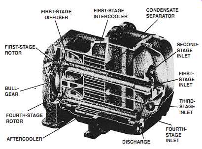
FIG. 6 Cutaway of bullgear centrifugal compressor.
Bullgear. The bullgear centrifugal compressor ( FIG. 6) is a multistage unit that uses a large helical gear mounted onto the compressor's driven shaft and two or more pinion gears, which drive the impellers. These impellers act in series, whereby com pressed air or gas from the first-stage impeller discharge is directed by flow channels within the compressor's housing to the second-stage inlet. The discharge of the second stage is channeled to the inlet of the third stage. This channeling occurs until the air or gas exits the final stage of the compressor.
Generally, the driver and bullgear speed is 3,600 rpm or less, and the pinion speeds are as high as 60,000 rpm (see FIG. 7). These machines are produced as a package, with the entire machine-train mounted on a common foundation that also includes a panel with control and monitoring instrumentation.
Positive Displacement:
Positive-displacement compressors, also referred to as dynamic-type compressors, confine successive volumes of fluid within a closed space. The pressure of the fluid increases as the volume of the closed space decreases. Positive-displacement compressors can be reciprocating or screw-type.
Reciprocating. Reciprocating compressors are positive-displacement types having one or more cylinders. Each cylinder is fitted with a piston driven by a crankshaft through a connecting rod. As the name implies, compressors within this classification displace a fixed volume of air or gas with each complete cycle of the compressor.
Reciprocating compressors have unique operating dynamics that directly affect their vibration profiles. Unlike most centrifugal machinery, reciprocating machines combine rotating and linear motions that generate complex vibration signatures.
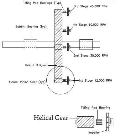
FIG. 7 Internal bullgear drive's pinion gears at each stage. Helical Gear.
Crankshaft frequencies. All reciprocating compressors have one or more crank shaft(s) that provide the motive power to a series of pistons, which are attached by piston arms. These crankshafts rotate in the same manner as the shaft in a centrifugal machine; however, their dynamics are somewhat different. The crankshafts generate all of the normal frequencies of a rotating shaft (i.e., running speed, harmonics of running speed, and bearing frequencies), but the amplitudes are much higher.
In addition, the relationship of the fundamental (1X) frequency and its harmonics changes. In a normal rotating machine, the 1X frequency normally contains between 60 and 70 percent of the overall, or broadband, energy generated by the machine-train.
In reciprocating machines, however, this profile changes. Two-cycle reciprocating machines, such as single-action compressors, generate a high second harmonic (2X) and multiples of the second harmonic. While the fundamental (1X) is clearly present, it’s at a much lower level.
Frequency shift caused by pistons. The shift in vibration profile is the result of the linear motion of the pistons used to provide compression of the air or gas. As each piston moves through a complete cycle, it must change direction two times.
This reversal of direction generates the higher second harmonic (2X) frequency component.
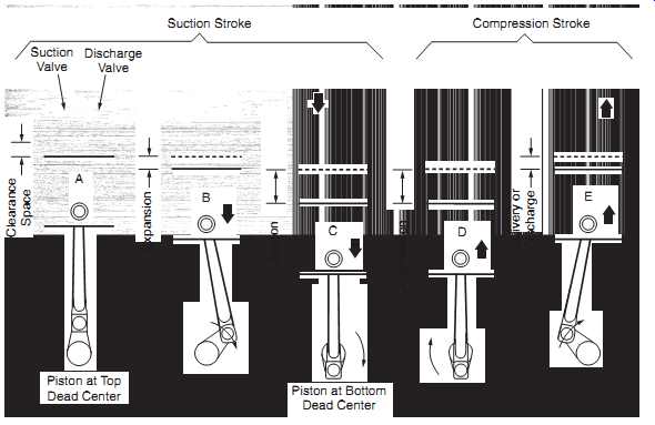
FIG. 8 Two-cycle, or single-action, air compressor cylinders. Piston
at Bottom Dead Center Piston at Top Dead Center Suction Stroke Suction
Valve Discharge Valve Compression Stroke
In a two-cycle machine, all pistons complete a full cycle each time the crankshaft completes one revolution. FIG. 8 illustrates the normal action of a two-cycle, or single-action, compressor. Inlet and discharge valves are located in the clearance space and connected through ports in the cylinder head to the inlet and discharge connections.
During the suction stroke, the compressor piston starts its downward stroke and the air under pressure in the clearance space rapidly expands until the pressure falls below that on the opposite side of the inlet valve (Point B). This difference in pressure causes the inlet valve to open into the cylinder until the piston reaches the bottom of its stroke (Point C).
During the compression stroke, the piston starts upward, compression begins, and at Point D has reached the same pressure as the compressor intake. The spring-loaded inlet valve then closes. As the piston continues upward, air is compressed until the pressure in the cylinder becomes great enough to open the discharge valve against the pressure of the valve springs and the pressure of the discharge line (Point E). From this point, to the end of the stroke (Point E to Point A), the air compressed within the cylinder is discharged at practically constant pressure.
The impact energy generated by each piston as it changes direction is clearly visible in the vibration profile. Because all pistons complete a full cycle each time the crank shaft completes one full revolution, the total energy of all pistons is displayed at the fundamental (1X) and second harmonic (2X) locations. In a four-cycle machine, two complete revolutions (720 degrees) are required for all cylinders to complete a full cycle.
Piston orientations. Crankshafts on positive-displacement reciprocating compressors have offsets from the shaft centerline that provide the stroke length for each piston.
The orientation of the offsets has a direct effect on the dynamics and vibration amplitudes of the compressor. In an opposed-piston compressor where pistons are 180 degrees apart, the impact forces as the pistons change directions are reduced. As one piston reaches top dead center, the opposing piston also is at top dead center. The impact forces, which are 180 degrees out-of-phase, tend to cancel out or balance each other as the two pistons change directions.
Another configuration, called an unbalanced design, has piston orientations that are neither in-phase nor 180 degrees out-of-phase. In these configurations, the impact forces generated as each piston changes direction are not balanced by an equal and opposite force. As a result, the impact energy and the vibration amplitude are greatly increased.
Horizontal reciprocating compressors (see FIG. 9) should have X-Y data points on both the inboard and outboard main crankshaft bearings, if possible, to monitor the connecting rod or plunger frequencies and forces.
Screw. Screw compressors have two rotors with interlocking lobes and act as positive-displacement compressors (see Figure 10). This type of compressor is designed for baseload, or steady-state, operation and is subject to extreme instability if either the inlet or discharge conditions change. Two helical gears mounted on the outboard ends of the male and female shafts synchronize the two rotor lobes.
Analysis parameters should be established to monitor the key indices of the compressor's dynamics and failure modes. These indices should include bearings, gear mesh, rotor passing frequencies, and running speed; however, because of its sensitivity to process instability and the normal tendency to thrust, the most critical monitoring parameter is axial movement of the male and female rotors.
Bearings. Screw compressors use both Babbitt and rolling-element bearings. Because of the thrust created by process instability and the normal dynamics of the two rotors, all screw compressors use heavy-duty thrust bearings. In most cases, they are located on the outboard end of the two rotors, but some designs place them on the inboard end. The actual location of the thrust bearings must be known and used as a primary measurement-point location.
Gear mesh. The helical timing gears generate a meshing frequency equal to the number of teeth on the male shaft multiplied by the actual shaft speed. A narrowband window should be created to monitor the actual gear mesh and its modulations. The limits of the window should be broad enough to compensate for a variation in speed between full load and no load.
The gear set should be monitored for axial thrusting. Because of the compressor's sensitivity to process instability, the gears are subjected to extreme variations in induced axial loading. Coupled with the helical gear's normal tendency to thrust, the change in axial vibration is an early indicator of incipient problems.
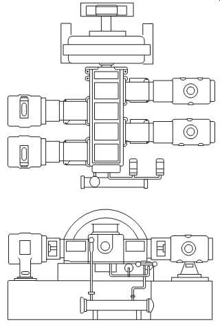
FIG. 9 Horizontal, reciprocating compressor.
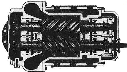
FIG. 10 Screw compressor-steady-state applications only.
Rotor passing. The male and female rotors act much like any bladed or gear unit. The number of lobes on the male rotor multiplied by the actual male shaft speed deter mines the rotor-passing frequency. In most cases, there are more lobes on the female than on the male. To ensure inclusion of all passing frequencies, the rotor-passing frequency of the female shaft also should be calculated. The passing frequency is equal to the number of lobes on the female rotor multiplied by the actual female shaft speed.
Running speeds. The input, or male, rotor in screw compressors generally rotates at a no-load speed of either 1,800 or 3,600 rpm. The female, or driven, rotor operates at higher no-load speeds ranging between 3,600 to 9,000 rpm. Narrowband windows should be established to monitor the actual running speed of the male and female rotors. The windows should have an upper limit equal to the no-load design speed and a lower limit that captures the slowest, or fully loaded, speed. Generally, the lower limits are between 15 and 20 percent lower than no-load.
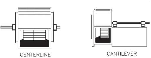
FIG. 11 Major fan classifications.
Fans
Fans have many different industrial applications and designs vary; however, all fans fall into two major categories: centerline and cantilever. The centerline configuration has the rotating element located at the midpoint between two rigidly supported bearings. The cantilever or overhung fan has the rotating element located outboard of two fixed bearings. FIG. 11 illustrates the difference between the two fan classifications.
The following parameters are monitored in a typical predictive maintenance program for fans: aerodynamic instability, running speeds, and shaft mode shape, or shaft deflection.
Aerodynamic Instability:
Fans are designed to operate in a relatively steady-state condition. The effective control range is typically 15 to 30 percent of their full range. Operation outside of the effective control range results in extreme turbulence within the fan, which causes a significant increase in vibration. In addition, turbulent flow caused by restricted inlet airflow, leaks, and a variety of other factors increases rotor instability and the overall vibration generated by a fan.
Both of these abnormal forcing functions (i.e., turbulent flow and operation outside of the effective control range) increase the level of vibration; however, when the instability is relatively minor, the resultant vibration occurs at the vane pass frequency. As it become more severe, the broadband energy also increases significantly.
A narrowband window should be created to monitor the vane-pass frequency of each fan. The vane-pass frequency is equal to the number of vanes or blades on the fan's rotor multiplied by the actual running speed of the shaft. The lower and upper limits of the narrowband should be set about 10 percent above and below (±10%) the calculated vane-pass frequency. This compensates for speed variations and includes the broadband energy generated by instability.
Running Speeds:
Fan running speed varies with load. If fixed filters are used to establish the bandwidth and narrowband windows, the running speed upper limit should be set to the synchronous speed of the motor, and the lower limit set at the full-load speed of the motor.
This setting provides the full range of actual running speeds that should be observed in a routine monitoring program.
Shaft Mode Shape (Shaft Deflection):
The bearing-support structure is often inadequate for proper shaft support because of its span and stiffness. As a result, most fans tend to operate with a shaft that deflects from its true centerline. Typically, this deflection results in a vibration frequency at the second (2X) or third (3X) harmonic of shaft speed.
A narrowband window should be established to monitor the fundamental (1X), second (2X), and third (3X) harmonic of shaft speed. With these windows, the energy associated with shaft deflection, or mode shape, can be monitored.
Generators
As with electric-motor rotors, generator rotors always seek the magnetic center of their casings. As a result, they tend to thrust in the axial direction. In almost all cases, this axial movement, or endplay, generates a vibration profile that includes the fundamental (1X), second (2X), and third (3X) harmonic of running speed. Key monitoring parameters for generators include bearings, casing and shaft, line frequency, and running speed.
Bearings:
Large generators typically use Babbitt bearings, which are non-rotating, lined metal sleeves (also referred to as fluid-film bearings) that depend on a lubricating film to prevent wear; however, these bearings are subjected to abnormal wear each time a generator is shut off or started. In these situations, the entire weight of the rotating element rests directly on the lower half of the bearings. When the generator is started, the shaft climbs the Babbitt liner until gravity forces the shaft to drop to the bottom of the bearing. This alternating action of climb and fall is repeated until the shaft speed increases to the point that a fluid-film is created between the shaft and Babbitt liner.
Subharmonic frequencies (i.e., less than the actual shaft speed) are the primary evaluation tool for fluid-film bearings, and they must be monitored closely. A narrowband window that captures the full range of vibration frequency components between electronic noise and running speed is an absolute necessity.
Casing and Shaft:
Most generators have relatively soft support structures. Therefore, they require shaft vibration-monitoring measurement points in addition to standard casing measurement points. This requires the addition of permanently mounted proximity, or displacement, transducers that can measure actual shaft movement.
The third (3X) harmonic of running speed is a critical monitoring parameter. Most, if not all, generators tend to move in the axial plane as part of their normal dynamics.
Increases in axial movement, which appear in the third harmonic, are early indicators of problems.
Line Frequency:
Many electrical problems cause an increase in the amplitude of line frequency, typically 60Hz, and its harmonics. Therefore, a narrowband should be established to monitor the 60, 120, and 180Hz frequency components.
Running Speed:
Actual running speed remains relatively constant on most generators. While load changes create slight variations in actual speed, the change in speed is minor. Generally, a narrowband window with lower and upper limits of ±10 percent of design speed is sufficient.
Process Rolls
Process rolls are commonly found in paper machines and other continuous process applications. Process rolls generate few unique vibration frequencies. In most cases, the only vibration frequencies generated are running speed and bearing rotational frequencies; however, rolls are highly prone to loads induced by the process. In most cases, rolls carry some form of product or a mechanism that, in turn, carries a product.
For example, a simple conveyor has rolls that carry a belt, which carries product from one location to another. The primary monitoring parameters for process rolls include bearings, load distribution, and misalignment.
Bearings:
Both non-uniform loading and roll misalignment change the bearing load zones. In general, either of these failure modes results in an increase in outer-race loading. This is caused by the failure mode forcing the full load onto one quadrant of the bearing's outer race. Therefore, the ball-pass outer-race frequency should be monitored closely on all process rolls. Any increase in this unique frequency is a prime indication of a load, tension, or misaligned roll problem.
Load Distribution:
By design, process rolls should be uniformly loaded across their entire bearing span (see FIG. 12). Improper tracking and/or tension of the belt, or product carried by the rolls, will change the loading characteristics.
The loads induced by the belt increase the pressure on the loaded bearing and decrease the pressure on the unloaded bearing. An evaluation of process rolls should include a cross-comparison of the overall vibration levels and the vibration signature of each roll's inboard and outboard bearing.
Misalignment:
Misalignment of process rolls is a common problem. On a continuous process line, most rolls are mounted in several levels. The distance between the rolls and the change in elevation make it extremely difficult to maintain proper alignment. In a vibration analysis, roll misalignment generates a signature similar to classical parallel mis alignment. It generates dominant frequencies at the fundamental (1X) and second (2X) harmonic of running speed.
Pumps
A wide variety of pumps is used by industry, which can be grouped into two types: centrifugal and positive displacement. Pumps are highly susceptible to process induced or installation-induced loads. Some pump designs are more likely to have axial- or thrust-induced load problems. Induced loads created by hydraulic forces also are a serious problem in most pump applications. Recommended monitoring for each type of pump is essentially the same, regardless of specific design or manufacturer; however, process variables such as flow, pressure, load, and so on must be taken into account.
Centrifugal:
Centrifugal pumps can be divided into two basic types: end-suction and horizontal split-case. These two major classifications can be further broken down into single stage and multistage. Each of these classifications has common monitoring parameters, but each also has unique features that alter their forcing functions and the resultant vibration profile. The common monitoring parameters for all centrifugal pumps include axial thrusting, vane-pass, and running speed.
Axial Thrusting. End-suction and multistage pumps with inline impellers are prone to excessive axial thrusting. In the end-suction pump, the centerline axial inlet configuration is the primary source of thrust. Restrictions in the suction piping, or low suction pressures, create a strong imbalance that forces the rotating element toward the inlet.
Multistage pumps with inline impellers generate a strong axial force on the outboard end of the pump. Most of these pumps have oversized thrust bearings (e.g., Kingsbury bearings) that restrict the amount of axial movement; however, bearing wear caused by constant rotor thrusting is a dominant failure mode. The axial movement of the shaft should be monitored when possible.
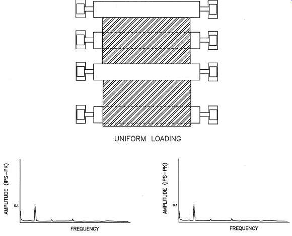
FIG. 12 Rolls should be uniformly loaded.
Hydraulic Instability ( Vane Pass). Hydraulic or flow instability is common in centrifugal pumps. In addition to the restrictions of the suction and discharge discussed previously, the piping configuration in many applications creates instability. Although flow through the pump should be laminar, sharp turns or other restrictions in the inlet piping can create turbulent flow conditions. Forcing functions such as these results in hydraulic instability, which displaces the rotating element within the pump.
In a vibration analysis, hydraulic instability is displayed at the vane-pass frequency of the pump's impeller. Vane-pass frequency is equal to the number of vanes in the impeller multiplied by the actual running speed of the shaft. Therefore, a narrowband window should be established to monitor the vane-pass frequency of all centrifugal pumps.
Running Speed. Most pumps are considered constant speed, but the true speed changes with variations in suction pressure and back-pressure caused by restrictions in the discharge piping. The narrowband should have lower and upper limits sufficient to compensate for these speed variations. Generally, the limits should be set at speeds equal to the full-load and no-load ratings of the driver.
There is a potential for unstable flow through pumps, which is created by both the design-flow pattern and the radial deflection caused by back-pressure in the discharge piping. Pumps tend to operate at their second-mode shape or deflection pattern. This operation mode generates a unique vibration frequency at the second harmonic (2X) of running speed. In extreme cases, the shaft may be deflected further and operate in its third (3X) mode shape. Therefore, both of these frequencies should be monitored.
Positive Displacement:
A variety of positive-displacement pumps is commonly used in industrial applications.
Each type has unique characteristics that must be understood and monitored; however, most of the major types have common parameters that should be monitored.
With the exception of piston-type pumps, most of the common positive-displacement pumps use rotating elements to provide a constant-volume, constant-pressure output.
As a result, these pumps can be monitored with the following parameters: hydraulic instability, passing frequencies, and running speed.
Hydraulic Instability ( Vane Pass). Positive-displacement pumps are subject to flow instability, which is created either by process restrictions or by the internal pumping process. Increases in amplitude at the passing frequencies, as well as harmonics of both shafts' running speed and the passing frequencies, typically result from instability.
Passing Frequencies. With the exception of piston-type pumps, all positive displacement pumps have one or more passing frequencies generated by the gears, lobes, vanes, or wobble-plates used in different designs to increase the pressure of the pumped liquid. These passing frequencies can be calculated in the same manner as the blade or vane-passing frequencies in centrifugal pumps (i.e., multiplying the number of gears, lobes, vanes, or wobble plates times the actual running speed of the shaft).
Running Speeds. All positive-displacement pumps have one or more rotating shafts that provide power transmission from the primary driver. Narrowband windows should be established to monitor the actual shaft speeds, which are in most cases essentially constant. Upper and lower limits set at ±10 percent of the actual shaft speed are usually sufficient.