The case for buying a new machine tool, or setting up an extra production line, can be assessed in this way and is the normal basis on which a business is set up or expanded. The purchase price plus installation, recruitment, and training costs must be paid off within a limited number of years and continue to show a substantial profit after deducting the amount of borrowed capital, operating cost, and so on; however, the benefits from an investment in a condition monitoring (CM) system are more difficult to assess, especially as a simple cost-benefit exercise, because, to put it simply, the variables are much more intuitive and less measurable than pure machine performance characteristics.
The ultimate justification for a CM system is where a bottleneck machine is totally dependent on a single component such as a bearing or gearbox, and failure of this component would create a prolonged, unscheduled stoppage affecting large areas of the plant. The cost of such an event could well be in the six- figure bracket, and the effect on sales and customer satisfaction beyond quantification. Yet a convincing financial case depends largely on knowing how often this sort of disaster is likely to happen and having a precise knowledge of the non-quantifiable factors referred to earlier. At best, whatever the cost, if it were likely to happen, it would be foolish not to install some method of predicting it, so that the appropriate preventive action could be taken.
ASSESSING THE NEED FOR CONDITION MONITORING
Any maintenance engineer's assessment of plant condition is influenced by a variety of practical observations and analyses of machine performance data, such as the following:
- Frequency of breakdowns
- Randomness of breakdowns
- Need for repetitive repairs
- Number of defective products produced
- Potential dangers linked to poor performance
- Any excessive fuel consumption during operation
- Any reduced throughput during operation
These, and many more pointers, may suggest that a particular item of plant requires either careful monitoring, routine planned preventive maintenance, better emergency repair procedures, or some combination of all these approaches to ensure a reason able level of operational availability. The engineering symptoms can, however, rarely be quantified accurately in terms of financial loss. Very few companies can put an accurate figure on the cost of downtime per hour. Many have no reliable records of their aggregate downtime at all, even if they could put a value per hour on it.
Thus, although a maintenance engineer may decide that a particular machine with a history of random bearing failures requires CM, if problems are to be anticipated, and the plant should be taken out of use before a catastrophic in-service failure occurs, how can he or she justify the expenditure of, say, $10,000 on the appropriate monitoring equipment, when plant and production records may be too vague to show what time and expense could be saved, and what this savings represents in terms of profit and loss to the company? This dilemma can be a daily occurrence for engineering and maintenance staffs in large and small companies throughout the country.
As if the practical problems of quantifying both the potential losses and gains were not difficult enough, the status of maintenance engineering in many organizations is such that any financial justification, however accurate, can be meaningless. The maintenance department in most companies is usually classified as a cost overhead. This means that a fixed sum is allocated to maintenance each year as a budget, which covers the cost of staff wages, spare parts, consumable items, and so on. The maintenance department is then judged for performance, financially or on its ability to work within its budget. Overspending is classified as "bad," and may result in restricting the department's resources even further in future years, whereas under-spending is classified as "good," in that it contributes directly to company profits, even if equipment maintenance is neglected and manufacturing quality or throughput suffers as a result.
Let us suppose that a forward-looking engineer succeeds in persuading his or her financial director-who knows nothing about CM and would rather invest the money anyway-to part with the capital needed to buy the necessary CM equipment. What happens then? Our hero, by using CM, succeeds in reducing unscheduled machine stoppages drastically, but which department gets the credit? Usually production because they have not needed to work overtime to make up for any lost production or have fewer rejects. Alternately, the sales department may receive the credit because of improved product quality or reduced manufacturing cost, which has given them an advantage over the firm's competitors. The maintenance engineer is rarely recognized as having added to the organization's improved cash flow by his or her actions.
Thus, a company that does not have a system of standard value costing cannot hope to isolate the benefits of efficient plant engineering and persuade the board of directors to invest in an effective arrangement for equipment purchasing and maintenance.
This presents a bleak picture for the person who has to make out a good financial case for installing a particular CM technique. Yet my company has seen this familiar situation repeatedly. This scenario occurs in most organizations, where we have received initial inquiries regarding installation of our software.
The expense of a computer system , for example, to collect and analyze plant data, without which an accurate cost justification is impossible, is often treated as nonproductive overhead. This is a classic Catch-22 situation, which has been stated in the past as: "We need the computer system to calculate whether we need the computer system, even though we know that it’s essential before we start." So, in order to justify the cost of a particular CM project, the appropriate person in the financial control hierarchy needs to be persuaded that the CM system should be treated as a capital investment charge in its own right, and not as an item of expenditure from the maintenance department's annual budget. Obviously, this will place the project in competition with other capital investment projects for the organization's limited resources. Accordingly, the case for justifying any CM equipment must be good and show a tangible return in a short period.
=========
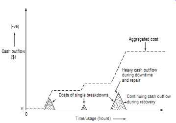
Fig. 1 Typical cash flow diagram illustrating the cost of lost production.
Aggregated cost Heavy cash outflow during downtime and repair Continuing cash outflow during recovery Costs of single breakdowns Time/usage (hours) (-ve) Cash outflow
==========
COST JUSTIFICATION
To produce a good case for financial investment in CM equipment, it’s therefore important to obtain reliable past performance data for the plant under review. In addition, information relating to other equipment, whose operations may be improved by better performance from the plant whose failures we hope to prevent, must also be gathered. It’s also essential to establish an effective financial record of actual CM achievement. This is especially true after the installation of any original equipment, so that it’s possible to build on the success of an initial project.
The performance data relating to CM must therefore be quantified financially, which in effect can mean persuading the managers for all departments involved to estimate the cost of the various factors that fall within their responsibility. Many managers, who may have criticized maintenance engineering in the past for poor production plant performance, by statements such as: "It’s costing the company a fortune," can suddenly become reluctant to put an actual cost value on the loss, particularly when asked for precise data. It’s in their interest to try, however, because without financial data there can be no satisfactory cost justification for CM, and hence no will or investment to improve the maintenance situation. Ultimately, their department and the company will be the losers if poor maintenance leads to an uncompetitive marketplace position.
Some of the factors relevant to maintenance engineering that can have an adverse effect on the company's cash flow are as follows: Lost production and the need to work overtime to make up any shortfall in output; some organizations will find this factor relatively easy to quantify. For example, an unscheduled stoppage of 3 hours could mean 500 components not made, plus another 200 damaged during machine stoppage and restart. The production line would perhaps have to work an extra half shift of overtime to make up the loss, and thereby incur all the associated labor, heating, and other facility support costs involved. Alternately, the cost of a subcontract outside the company to make good the lost production is usually obtainable as a precise figure.
This figure is normally easy to obtain and in real expenditure terms, as opposed to the internal cost of working overtime, which may not be so precisely calculated.
Other costs may also be difficult to quantify accurately, such as the sales department's need to put a value on the cost of customer dissatisfaction if a delivery is delayed, or the cost of changing the production schedule to correct the loss in production if the particular product involved has a high priority. The cost of lost production is a random set of peaks in the cash flow diagram, as shown in Fig. 1. If treated independently, this cost can appear as a minor problem, but if aggregated the result can be quite startling. Even if we are able to accurately calculate the cost of lost production, however, we are still left with estimating the frequency and duration of future break downs, before we can come up with a cash flow statement.
Accordingly, it’s important to have good past records if we are to do any better than guess at a value. If breakdowns are purely random occurrences, then past records are not going to give us the ability to predict precise savings for inclusion in a sound financial case. They may, however, give a feel for the likely cost when a breakdown happens. At best, we could say , for example, the likely cost of a stoppage is $8,000 per hour, and likely breakdown duration is going to be two shifts at a minimum. The question senior management then has to face is: "Are you willing to spend $10,000 on this condition monitoring device or not?"
Poor-Quality Product as Plant Performance Deteriorates:
As a machine's bearings wear out, its lubricants decay, or its flow rates fluctuate, the product being manufactured may suffer damage. This can lead to an increase in the level of rejects or to growing customer dissatisfaction regarding product quality.
Financial quantification here is similar to that outlined previously but can be even less precise because the total effect of poor quality may be unknown. In a severe case, the loss of ISO-9000 certification may take place, which can have financial implications well beyond any caused by increased rejection rates.
Increased Cost of Fuel and Other Consumables as the Plant Condition Deteriorates:
A useful example of this point is the increased fuel consumption as boilers approach their time for servicing. The cost associated with servicing can be quantified precisely from past statistics or a service supplier's data. The damaging effects of a vibrating bearing or gearbox are, however, less easy to quantify directly and even more so as one realizes that they can have further consequential effects that compound the total cost. For example, the vibration in a faulty gearbox could in turn lead to rapid wear on clutch plates, brake linings, transmission bushes, or conveyor belt fabric. Thus, the component replacement costs rise, but maintenance records won’t necessarily relate this situation to the original gearbox defect. Fig. 2 shows how the cost of deterioration in plant condition rises as the equipment decays, with the occasional sudden or gradual increases as the consequential effects add to overall costs.
===
Condition deteriorating Time/usage (hours) (-ve) Cash outflow ( )
0 Plant in good condition Extra cost due to knock-on effect Increasing consumption of fuel, spares, etc.
Steady cost of fuel, spares, etc.
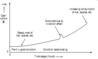
Fig. 2 Typical cost of deterioration in plant condition.
Time/usage (hours) (-ve) Cash outflow ( ) 0
Cost of routine ppm Increasing cost as major components begin to fail Increasing wear on moving parts Plant 'as new' S Fig. 3 Typical cost of a preventive maintenance strategy.
===
Cost of Current Maintenance Strategy:
The cost of a maintenance engineering department as a whole should be fairly clearly documented, including wages, spares, overheads, and so on; however, it’s usually difficult to break this cost down into individual plant items and virtually impossible to allocate an accurate proportion of this total cost to a single component's maintenance.
In addition, overall costs will rise steadily in respect to routine plant maintenance as the equipment deteriorates with age and needs more careful attention to keep it running smoothly. Fig. 3 outlines the cost of a current planned preventive maintenance strategy and shows it to be a steady outflow of cash for labor and spares, increasing as the plant ages.
If CM is to replace planned preventive maintenance, considerable savings may be realized in the spares and labor requirement for the plant, which may be found to be over maintained. This is more common than one might expect because maintenance has always believed that regular prevention is much less costly than a serious breakdown in service. Unit replacement at weekends or during a stop period is not reflected in lost production figures, and the cost of stripping and refurbishing the plant is often lost in the maintenance department's wage budget for the year. In other words, the cost of planned preventive maintenance on plant and equipment can be a constant drain on resources that goes undetected. Accordingly, it should really be made avail able for comparison with the cost of monitoring the unit's condition on a regular basis and applying corrective measures only when needed.
JUSTIFYING PREDICTIVE MAINTENANCE
In general, the cost of any current maintenance position is largely vague and unpredictable. This is true even if enough data are available to estimate past expenditure and allocate this precisely to a particular plant item. Thus, if we are to make any sense of financial justification, we must somehow overcome this impasse. The reduced cost of maintenance is usually the first factor that a financial manager looks at when we present our case, even though the real but intangible savings come from reduced down time. Ideally, past worksheets should give the aggregated maintenance hours spent on the plant. These can then be pro-rated against total labor costs. Similarly, the spares consumption recorded on the worksheets can be multiplied by unit costs. The cost of the maintenance strategy for the plant will then be the labor cost plus the spares cost plus an overhead element.
Unfortunately, the nearest we are likely to get to a value for maintenance overheads will be to take the total maintenance department's overhead value and multiply it by the plant's maintenance labor cost, divided by the total maintenance labor cost. Even if we manage to arrive at a satisfactory figure, its justification will be queried if we cannot show it as a tangible savings, either resulting from reduced staffing levels in the maintenance department or through reduced spares consumption, which would also be acceptable as a real savings. The estimates will need to be aggregated and grouped according to how they can be allocated (e.g., whether they are downtime based, total cost per hour the plant is stopped, frequency-based, recovery cost per breakdown, or general cost of regaining customer orders and confidence after failure to deliver). By using these estimates, plus the performance data that have been collected, it should then be possible to estimate the cost of machine failure and poor performance during the past few years or months. In addition, it should also be possible to allocate a probable savings if machine performance is improved by a realistic amount.
It may even be possible to create a traditional cash flow diagram showing expenses against savings and the final breakeven point, although its apparent precision is much less than the quality of the data would suggest. If we aggregate the graphs for the cost of the current maintenance situation, and plot that alongside the expected costs after installing CM, as shown in Fig. 4, then the area between the two represents the potential savings. Fig. 5, conversely, shows how the cost of installing CM equipment is high at first, until the capital has been paid off, and then the operating cost becomes fairly low but steady during the life of the CM equipment.
Put against the savings, there will be both the capital and running costs of introducing a CM project to be considered, which are outlined as follows.
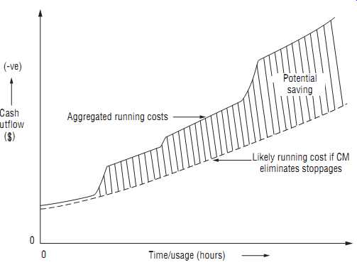
Fig. 4 Typical potential savings produced by use of condition monitoring.
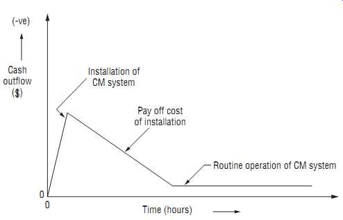
Fig. 5 Typical cost of condition monitoring installation and operation.
Installation Cost:
Some of the capital cost will be clearly defined by the equipment price and any specialist installation cost. There may also be preliminary alterations required, such as creating access, installing foundations, covering or protection, power supply, service access, and so on. Some or all may be subject to development grants or other financial inducement, as may the cost of consultancy before, during, or after the installation. This could well include the cost of producing a financial project justification. The cost of lost production during installation may be avoided if the equipment is installed during normal product changes or shutdown periods; however, in a continuous process this may be another overhead to be added to the initial capital investment. Finally, it may be necessary to send staff to a training course, which has not been included in the equipment price. The cost of staff time and the course itself may be offset by training grants in some areas, which should be investigated. It’s also possible that the vendor will offer rental terms on the CM equipment, in which case the cost becomes part of the operating rather than the capital budget.
Operating Cost:
Once the unit has been installed and commissioned, the major cost is likely to be its staffing requirement. If the existing engineering staff has sufficient skill and training, and the improved plant performance reduces their workload sufficiently, then operating the equipment and monitoring its results may be absorbed without additional cost.
In our experience, this time-saving factor has often been ignored in justifying the case for improved maintenance techniques. In retrospect, however, it has proved to be one of the main benefits of installing a computer-based monitoring system.
For example, a cable maker found that his company had increased its plant capacity by 50 percent during the year after the introduction of computer-based maintenance.
Yet the level of maintenance staff needed to look after the plant had remained unchanged. This amounted to a 60 percent improvement in overall productivity.
Another example of this effect was a drinks manufacturer who used a computerized scheduler to change from time-based to usage-based maintenance. This was done because demands on production fluctuated rapidly with changes in the weather. As a result, the workload on the maintenance trades fell so far that they were able to maintain an additional production line without any staffing increase at all.
If these savings can be made by better scheduling, how much more improvement in labor availability would there be if maintenance could be related to a measurable plant condition, and the servicing planned to coincide with a period of low activity in the production or maintenance schedule? So, the ongoing cost of labor needed to run the CM project must be assessed carefully and balanced against the potential labor savings as performance improves. Other continuing costs must also be considered, such as the fuel or consumables needed by the unit; however, these costs are normally small, and recent trends have shown that consumable costs tend to decrease as more companies turn to this type of equipment.
Combining the aforementioned initial costs and savings should result in an early outflow of cash investment in equipment and training, but this soon crosses the breakeven point within an acceptable period. It should then level off into a steady profit, which represents a satisfying return on the initial investment, as reduced maintenance costs, plus improved equipment performance, are realized as overall financial gains. Fig. 6 indicates how the cash flow from investment in CM moves through the breakeven point into a region of steady positive financial gain.
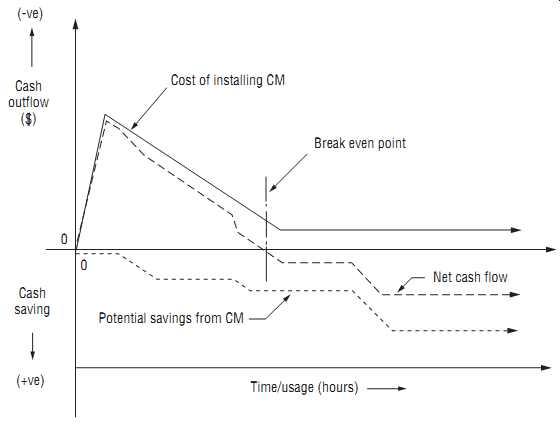
Fig. 6 Typical overall cash flow from an investment in predictive maintenance.
Conclusions:
In conclusion, it’s possible to say that the financial justification for installation of any item of CM equipment should based on a firm business plan, where investment cost is offset by quantified financial benefits; however, the vagueness of the factors avail-able for quantification, the lack of firm tangible benefits, and the financial environment in which maintenance engineers operate all conspire to make the construction of such a plan difficult.
Until the engineer is given the facilities to collect and analyze performance data accurately and consistently; until the engineering and manufacturing departments are integrated under a precise standard value-costing system; and until the maintenance engineering function is given the status of a profit center, then financial justification will never become the precise science it should be. Instead, the more normal process is one in which an engineer makes a decision to install a CM system and then backs it up with precise-looking figures based on imprecise data. Fortunately, once the improved system has been approved, its performance is only rarely monitored against that estimated in the original business plan. This is largely because the financial values or benefits achieved are even more difficult to extract and quantify in a post installation audit than those in the original business plan.
ECONOMICS OF PREVENTIVE MAINTENANCE
Maintenance is, and should be, managed like a business; however, few maintenance managers have the basic skill and experience needed to understand the economics of an effective business enterprise. This section provides a basic understanding of maintenance economics.
Benefits versus Costs:
Preventive maintenance is an investment. Like anything in which we invest money and resources, we expect to receive benefits from preventive maintenance that are greater than our investment. The following financial overview is intended to provide enough knowledge to know what method is best and what the financial experts will need to know to provide assistance.
Making preventive investment trade-offs requires consideration of the time-value of money. Whether the organization is profit-driven, not-for-profit, private, public, or government, all resources cost money. The three dimensions of payback analysis are (1) the money involved in the flow, (2) the period over which the flow occurs, and (3) the appropriate cost of money expected over that period.
Preventive maintenance analysis is usually either "Yes/No" or choosing one of several alternatives. With any financial inflation, which is the time we live in, the time-value of money means that a dollar in your pocket today is worth more than that same dollar a year from now. Another consideration is that forecasting potential outcomes is much more accurate in the short term than it’s in the long term, which may be several years away. Decision-making methods include the following:
- Payback
- Percent rate of return (PRR)
- Average return on investment (ROI)
- Internal rate of return (IRR)
- Net present value (NPV)
- Cost-benefit ratio (CBR)
The corporate controller often sets the financial rules to be used in justifying capital projects. Companies have rules like, "Return on investment must be at least 20 percent before we will even consider a project" or "Any proposal must pay back within 18 months." Preventive maintenance evaluations should normally use the same set of rules for consistency and to help achieve management support. It’s also important to realize that the political or treasury drivers behind those rules may not be entirely logical for your level of working decision.
Payback:
Payback simply determines the number of years that are required to recover the original investment. Thus, if you pay $50,000 for a test instrument that saves downtime and increases production worth $25,000 a year, then the payback is:
This concept is easy to understand. Unfortunately, it disregards the fact that the $25,000 gained the second year may be worth less than the $25,000 gained this year because of inflation. It also assumes a uniform stream of payback, and it ignores any returns after the two years. Why two years instead of any other number? There may be no good reason except "The controller says so." It should also be noted that if simple payback is negative, then you probably don’t want to make the investment.
Percent Rate of Return (PRR):
Percent rate of return is a close relation of payback that is the reciprocal of the payback period. In our case above:
This is often called the naive rate of return because, like payback, it ignores the cost of money over time, compounding effect, and logic for setting a finite time period for payback.
Return on Investment (ROI):
Return on investment is a step better because it considers depreciation and salvage expenses and all benefit periods. If we acquire a test instrument for $80,000 that we project to have a five-year life, at which time it will be worth $5,000, then the cost calculation, excluding depreciation, is:
If we can benefit a total of $135,000 over that same five years, then the average increment is:
The average annual ROI is:
Ask your accounting firm how they handle depreciation because that expense can make a major difference in the calculation.
Internal Rate of Return (IRR):
Internal rate of return is more accurate than the preceding methods because it includes all periods of the subject life, considers the costs of money, and accounts for differing streams of cost and/or return over life. Unfortunately, the calculation requires a computer spreadsheet macro or a financial calculator. Ask your controller to run the numbers.
Net Present Value (NPV):
Net present value has the advantages of IRR and is easier to apply. We decide what the benefit stream should be by a future period in financial terms. Then we decide what the cost of capital is likely to be over the same time and discount the benefit stream by the cost of capital. The term net is used because the original investment cost is subtracted from the resulting present value for the benefit. If the NPV is positive, you should do the project. If the NPV is negative, then the costs outweigh the benefits.
Table 5 Capital Recovery, Uniform Series with Present Value $1
Cost-Benefit Ratio (CBR):
The cost-benefit ratio takes the present value (initial project cost + NPV) divided by the initial project cost. For example, if the project will cost $250,000 and the NPV is ...
$350,000, then:
It may appear that the CBR is merely a mirror of the NPV. The valuable addition is that CBR considers the size of the financial investment required. For example, two competing projects could have the same NPV, but if one required $1 million and the other required only $250,000, that absolute amount might influence the choice.
Compare the previous example with the $1 million example:
There should be little question that you would take the $250,000 project instead of the $1 million choice. Tables 2-1 through 2-5 provide the factors necessary for evaluating how much an investment today must earn over the next three years in order to achieve a target ROI. This calculation requires that we make a management judgment on what the inflation/interest rate will be for the payback time and what the pattern of those paybacks will be.
For example, if we spend $5,000 today to modify a machine in order to reduce break downs, the payback will come from improved production revenues, reduced maintenance labor, having the right parts, tools, and information to do the complete job, and certainly less confusion.
The intention of this brief discussion of financial evaluation is to identify factors that should be considered and to recognize when to ask for help from accounting, control, and finance experts. Financial evaluation of preventive maintenance is divided generally into either single transactions or multiple transactions. If payment or cost reductions are multiple, they may be either uniform or varied. Uniform series are the easiest to calculate. Non-uniform transactions are treated as single events that are then summed together.
Tables 1 through 5 are done in periods and interest rates that are most applicable to maintenance and service managers. The small interest rates will normally be applicable to monthly events, such as 1 percent per month for 24 months. The larger interest rates are useful for annual calculations. The factors are shown only to three decimal places because the data available for calculation are rarely even that accurate.
The intent is to provide practical, applicable factors that avoid overkill. If factors that are more detailed, or different periods or interest rates, are needed, they can be found in most economics and finance texts or automatically calculated by the macros in computerized spreadsheets. The future value factors (Tables1 and 3) are larger than 1, as are present values for a stream of future payments (Table 4). On the other hand, present value of a single future payment (Table 2) and capital recovery (Table 5 after the first year) result in factors of less than 1.000. The money involved to give the answer multiplies the table factor. Many programmable calculators can also work out these formulas. If , for example, interest rates are 15 percent per year and the total amount is to be repaid at the end of three years, refer to Table 1 on future value. Find the factor 1.521 at the intersection of three years and 15 percent. If our example cost is $35,000, it’s multiplied by the factor to give:
$35,000 x 1.521 = $53,235 due at the end of the term
Present values from Table 2-2 are useful to determine how much we can afford to pay now to recover, say, $44,000 in expense reductions over the next two years. If the interest rates are expected to be lower than 15 percent, then:
$44,000 x 0.75% = $33,264
Note that a dollar today is worth more than a dollar received in the future. The annuity tables are for uniform streams of either payments or recovery. Table 2-3 is used to determine the value of a uniform series of payments. If we start to save now for a future project that will start in three years, and save $800 per month through reduction of one person, and the cost of money is 1 percent per month, then $34,462 should be in your bank account at the end of 36 months.
$800 x 43.077 = $34,462
The factor 43.077 came from 36 periods at 1 percent. The first month's $800 earns interest for 36 months. The second month's savings earns for 35 months, and so on.
The use of factors is much easier than using single-payment tables and adding the amount for $800 earning interest for 36 periods ($1,114.80), plus $800 for 35 periods ($1,134.07), and continuing for 34, 33, and so on, through one. If I sign a purchase order for new equipment to be rented at $500 per month over five years at 1 percent per month, then:
$500 x 44.955 = $22,478
Note that five years is 60 months in the period column of Table 2-4. Capital recovery Table 2-5 gives the factors for uniform payments, such as mortgages or loans that repay both principal and interest. To repay $75,000 at 15 percent annual interest over five years, the annual payments would be:
$75,000 x 0.298 = $22,350
Note that over the five years, total payments will equal $111,750 (5 x $22,350), which includes the principal $75,000 plus interest of $36,750. Also note that a large difference is made by whether payments are due in advance or in arrears.
A maintenance service manager should understand enough about these factors to do rough calculations and then get help from financial experts for fine-tuning. Even more important than the techniques used is the confidence in the assumptions. Control and finance personnel should be educated in your activities so they will know what items are sensitive and how accurate (or best judgment) the inputs are, and will be able to support your operations.
Fig. 7 The relationship between cost and amount of preventive maintenance.
Trading Preventive for Corrective and Downtime
Fig. 7 illustrates the relationships between preventive maintenance, corrective maintenance, and lost production revenues. The vertical scale is dollars. The horizontal scale is the percentage of total maintenance devoted to preventive maintenance.
The percentage of preventive maintenance ranges from zero (no PMs) at the lower left intersection to nearly 100 percent preventive at the far right. Note that the curve does not go to 100 percent preventive maintenance because experience shows there will always be some failures that require corrective maintenance. Naturally, the more of any kind of maintenance that is done, the more it will cost to do those activities.
The trade-off, however, is that doing more preventive maintenance should reduce both corrective maintenance and downtime costs. Note that the downtime cost in this illustration is greater than either preventive or corrective maintenance. Nuclear power generating stations and many production lines have downtime costs exceeding $10,000 per hour. At that rate, the downtime cost far exceeds any amount of maintenance, labor, or even materials that we can apply to the job. The most important effort is to get the equipment back up without much concern for overtime or expense budget.
Normally, as more preventive tasks are done, there will be fewer breakdowns and therefore lower corrective maintenance and downtime costs. The challenge is to find the optimum balance point.
Fig. 8 Preventive maintenance, condition monitoring, and lost revenue cost, $000.
As shown in Fig. 7, it’s better to operate in a satisfactory region than to try for a precise optimum point. Graphically, every point on the total-cost curve represents the sum of the preventive costs plus corrective maintenance costs plus lost revenues costs.
If you presently do no preventive maintenance tasks at all, then each dollar of effort for preventive tasks will probably gain savings of at least $10 in reduced corrective maintenance costs and increased revenues. As the curve shows, increasing the investment in preventive maintenance will produce increasingly smaller returns as the breakeven point is approached. The total-cost curve bottoms out, and total costs begin to increase again beyond the breakeven point. You may wish to experiment by going past the minimum-cost point some distance toward more preventive tasks. Even though costs are gradually increasing, subjective measures, including reduced confusion, safety, and better management control, that don’t show easily in the cost calculations are still being gained with the increased preventive maintenance. How do you track these costs? Fig. 8 shows a simple record-keeping spreadsheet that helps keep data on a month-by-month basis.
It should be obvious that you must keep cost data for all maintenance efforts in order to evaluate financially the cost and benefits of preventive versus corrective maintenance and revenues. A computerized maintenance information system is best, but data can be maintained by hand for smaller organizations. One should not expect immediate results and should anticipate some initial variation. This delay could be caused by the momentum and resistance to change that is inherent in every electromechanical system, by delays in implementation through training and getting the word out to all personnel, by some personnel who continue to do things the old way, by statistical variations within any equipment and facility, and by data accuracy.
If you operate electromechanical equipment and presently don’t have a preventive maintenance program, you are well advised to invest at least half of your maintenance budget for the next three months in preventive maintenance tasks. You are probably thinking: "How do I put money into preventive and still do the corrective maintenance?" The answer is that you can't spend the same money twice. At some point, you have to stand back and decide to invest in preventive maintenance that will stop the large number of failures and redirect attention toward doing the job right once.
This will probably cost more money initially as the investment is made. Like any other investment, the return is expected to be much greater than the initial cost.
One other point: it’s useless to develop a good inspection and preventive task schedule if you don't have the people to carry out that maintenance when required. Careful attention should be paid to the Mean Time to Preventive Maintenance (MTPM). Many people are familiar with Mean Time to Repair (MTTR), which is also the Mean Corrective Time (M - ct). It’s interesting that the term MTPM is not found in any textbooks the author has seen, or even in the author's own previous writings, although the term M - pt is in use. It’s easier simply to use Mean Corrective Time (M - ct) and Mean Preventive Time (M - pt).
PM Time/Number of preventive maintenance events calculates M - pt. That equation may be expressed in words as the sum of all preventive maintenance time divided by the number of preventive activities done during that time. If , for example, five oil changes and lube jobs on earthmovers took 1.5, 1, 1.5, 2, and 1.5 hours, the total is 7.5 hours, which divided by the five events equals an average of 1.5 hours each. A few main points, however, should be emphasized here:
1. Mean Time Between Maintenance (MTBM) includes preventive and corrective maintenance tasks.
2. Mean Maintenance Time is the weighted average of preventive and corrective tasks and any other maintenance actions, including modifications and performance improvements.
3. Inherent Availability (Ai) considers only failure and M - ct. Achieved availability (Aa) adds in PM, although in a perfect support environment. Operational Availability (A0) includes all actions in a realistic environment.