AMAZON multi-meters discounts AMAZON oscilloscope discounts
For most rotating machines used in the process industries, the trend is toward higher speeds, higher horsepowers per machine, and less sparing.
The first of these factors increases the need for precise balancing and alignment. This is necessary to minimize vibration and premature wear of bearings, couplings, and shaft seals. The latter two factors increase the economic importance of high machine reliability, which is directly dependent on minimizing premature wear and breakdown of key components.
Balancing, deservedly, has long received attention from machinery manufacturers and users as a way to minimize vibration and wear. Many shop and field balancing machines, instruments, and methods have become available over the years. Alignment, which is equally important, has received proportionately less notice than its importance justifies.
Any kind of alignment, even straightedge alignment, is better than no alignment at all. Precise, two-indicator alignment is better than rough alignment, particularly for machines 3,600 rpm and higher. It can give greatly improved bearing and seal life, lower vibration, and better overall reliability. It does take longer, however, especially the first time it’s done to a particular machine, or when done by inexperienced personnel. The process operators and mechanical supervisors must be made aware of this time requirement. If they insist on having the job done in a hurry, they should do so with full knowledge of the likelihood of poor alignment and reduced machine reliability. FIG. 1 shows a serious machinery failure which started with piping-induced misalignment, progressed to coupling distress, bearing failure, and finally, total wreck.
Pre-alignment Requirements
The most important requirement is to have someone who knows what he is doing, and cares enough to do it right. Continuity is another important factor. Even with good people, frequent movement from location to location can cause neglect of things such as tooling completeness and pre alignment requirements.
The saying that " you can't make a silk purse out of a sow's ear" also applies to machinery alignment. Before undertaking an alignment job, it’s prudent to check for other deficiencies which would largely nullify the benefits or prevent the attainment and retention of good alignment. Here is a list of such items and questions to ask oneself:
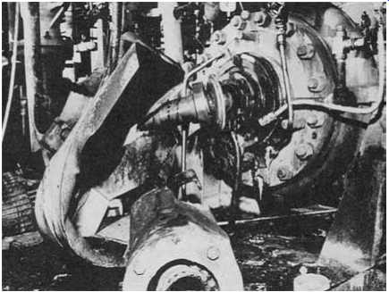
FIG. 1. Machinery damage caused by bearing seizure. Bearing seizure
was the result of gear coupling damage, and gear coupling damage was
caused by excessive misalignment, caused by piping forces.
Foundation
Adequate size and good condition? A rule of thumb calls for concrete weight equal to three times machine weight for rotating machines, and five times for reciprocating machines.
Grout
Suitable material, good condition, with no voids remaining beneath baseplate? Tapping with a small hammer can detect hollow spots, which can then be filled by epoxy injection or other means. This is a lot of trouble, though, and often is not necessary if the lack of grout is not causing vibration or alignment drift.
Baseplate
Designed for adequate rigidity? Machine mounting pads level, flat, parallel, coplanar, clean? Check with straight edge and feeler gauge. Do this upon receipt of new pumps, to make shop correction possible-and maybe collect the cost from the pump manufacturer. Shims clean, of adequate thickness, and of corrosion- and crush-resistant material? If commercial pre-cut shims are used, check for actual versus marked thicknesses to avoid a soft foot condition.
Machine hold-down bolts of adequate size, with clearance to permit alignment corrective movement? Pad height leaving at least 2 in. jacking clearance beneath center at each end of machine element to be adjusted for alignment? If jackscrews are required, are they mounted with legs sufficiently rigid to avoid deflection? Are they made of type 316 stainless steel, or other suitable material, to resist field corrosion? Water or oil cooled or heated pedestals are usually unnecessary, but can in some cases be used for onstream alignment thermal compensation.
Piping Is connecting piping well fitted and supported, and sufficiently flexible, so that no more than 0.003 in. vertical and horizontal (measured separately-not total) movement occurs at the flexible coupling when the last pipe flanges are tightened? Selective flange bolt tightening may be required, while watching indicators at the coupling. If pipe
flange angular misalignment exists, a "dutchman" or tapered filler piece may be necessary. To determine filler piece dimensions, measure flange gap around circumference, then calculate as follows:
1/8 in Max Gap Min Gap Gasket OD Flange OD Maximum Thickness of Tapered Filler Piece
1/8 in. = Dutchman Minimum Thickness (180° from Maximum Thickness). Dutchman OD and ID same as gasket OD and ID.
Spiral wound gaskets may be helpful, in addition to or instead of a tapered filler piece. Excessive parallel offset at the machine flange connection cannot be cured with a filler piece. It may be possible to absorb it by offsetting several successive joints slightly, taking advantage of clearance between flange bolts and their holes. If excessive offset remains, the piping should be bent to achieve better fit. For the "stationary" machine element, the piping may be connected either before or after the alignment is done-pro vided the foregoing precautions are taken, and final alignment remains within acceptable tolerances. In some cases, pipe expansion or movement may cause machine movement leading to misalignment and increased vibration. Better pipe supports or stabilizers may be needed in such situations. At times it may be necessary to adjust these components with the machine running, thus aligning the machine to get minimum vibration. Sometimes, changing to a more tolerant type of coupling, such as elastomeric, may help.
Coupling Installation -- Some authorities recommend installation on typical pumps and drivers with an interference fit, up to 0.0005 in. per in. of shaft diameter. In our experience, this can give problems in subsequent removal or axial adjustment. If an interference fit is to be used, we prefer a light one-say 0.0003 in. to 0.0005 in. overall, regardless of diameter. For the majority of machines operating at 3,600 rpm and below, you can install couplings with 0.0005 in. overall diametral clearance, using a setscrew over the keyway. For hydraulic dilation couplings and other non-pump or special categories, see manufacturers' recommendations or appropriate section of this text. Many times, high-performance couplings require interference fits as high as 0.0025 in. per in. of shaft diameter.
Coupling cleanliness, and for some types, lubrication, are important and should be considered. Sending a repaired machine to the field with its lubricated coupling-half unprotected, invites lubricant contamination, rusting, dirt accumulation, and premature failure. Lubricant should be chosen from among those recommended by the coupling manufacturer or a reputable oil company. Continuous running beyond two years is inadvisable without inspecting a grease lubricated coupling, since the centrifuging effects are likely to cause caking and loss of lubricity.
Certain lubricants, e.g., Amoco and Koppers coupling greases, are reported to eliminate this problem, but visual external inspection is still advisable to detect leakage. Continuous lube couplings are subject to similar problems, although such remedies as anti-sludge holes can be used to allow longer runs at higher speeds. By far the best remedy is clean oil, because even small amounts of water will promote sludge formation. Spacer length can be important, since parallel misalignment accommodation is directly proportional to such length.
Alignment Tolerances
Before doing an alignment job, we must have tolerances to work toward.
Otherwise, we won’t know when to stop. One type of "tolerance" makes time the determining factor, especially on a machine that is critical to plant operation, perhaps the only one of its kind. The operations superintendent may only be interested in getting the machine back on the line, fast. If his influence is sufficient, the job may be hurried and done to rather loose alignment tolerances. This can be unfortunate, since it may cause excessive vibration, premature wear, and early failure. This gets us back to the need for having the tools and knowledge for doing a good alignment job efficiently. So much for the propaganda-now for the tolerances.
Tolerances must be established before alignment, in order to know when to stop. Various tolerance bases exist. One authority recommends 1/2-mil maximum centerline offset per in. of coupling length, for hot running mis alignment. A number of manufacturers have graphs which recommend tolerances based on coupling span and speed. A common tolerance in terms of face-and-rim measurements is 0.003-in, allowable face gap difference and centerline offset. This ignores the resulting accuracy variation due to face diameter and spacer length differences, but works adequately for many machines.
Be cautious in using alignment tolerances given by coupling manufacturers. These are sometimes rather liberal and, while perhaps true for the coupling itself, may be excessive for the coupled machinery.
A better guideline is illustrated in FIG. 2, which shows an upper, absolute misalignment limit, and a lower, "don't exceed for good long term operation limit." The real criterion is the running vibration. If excessive, particularly at twice running frequency and axially, further alignment improvement is probably required. Analysis of failed components such as bearings, couplings, and seals can also indicate the need for improved alignment.
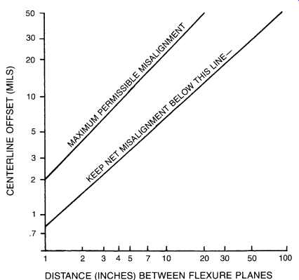
FIG. 2. Misalignment tolerances.
FIG. 2 can be applied to determine allowable misalignment for machinery equipped with nonlubricated metal disc and diaphragm couplings, up to perhaps 10,000 rpm. If the machinery is furnished with gear type couplings, FIG. 2 should be used up to 3,600 rpm only. At speeds higher than 3,600 rpm, gear couplings will tolerate with impunity only those shaft misalignments which limit the sliding velocity of engaging gear teeth to less than perhaps 120 in. per minute. For gear couplings, this velocity can be approximated by V = (pDN) tana, where:
D = gear pitch diameter, in.
N = revolutions per minute
2 tana= total indicator reading obtained at hub outside diameter, divided by distance between indicator planes on driver and driven equipment couplings.
Say, For example, we were dealing with a 3,560rpm pump coupled to a motor driven via a 6-in. pitch diameter gear coupling. We observe a total indicator reading of 26mils in the vertical plane and a total indicator reading of 12mils in the horizontal plane. The distance between the flexing member of the coupling, i.e., flexing member on driver and flexing member on driven machine, is 10in. The total net indicator reading is [(26) 2 + (12) 2] 1/2= 28.6mils. Tana (1/2)(28.6)/10) = 1.43mils/in., or 0.00143in./in. The sliding velocity is therefore [(p)(6)(3560)(0.00143)] = 96in. per minute.
Since this is below the maximum allowable sliding velocity of 120in. per minute, the installation would be within allowable misalignment.
Choosing an Alignment Measurement Setup
Having taken care of the preliminaries, we are now ready to choose an alignment setup, or arrangement of measuring instruments. Many such setups are possible, generally falling into three broad categories: face-and rim, reverse-indicator, and face-face-distance. The following sketches show several of the more common setups, numbered arbitrarily for ease of future reference. Note that if measurements are taken with calipers or ID micrometers, it may be necessary to reverse the sign from that which would apply if dial indicators are used.
Figures 3 through 8 show several common arrangements of indicators, jigs, etc. Other arrangements are also possible. For example, Figures 3 and 4 can be done with jigs, either with or without breaking the coupling. They can also sometimes be done when no spacer is present, by using right-angle indicator extension tips. Figures 6 and 7 can be set up with both extension arms and indicators on the same side, rather than 180° opposite as shown. In such cases, however, a sign reversal will occur in the calculations. Also, we can indicate on back of face, as for connected metal disc couplings. Again, a sign reversal will occur.
In choosing the setup to use, personal preference and custom will naturally influence the decision, but here are some basic guidelines to follow.
Reverse-Indicator Method
This is the setup we prefer for most alignment work. As illustrated in FIG. 9, it has several advantages:
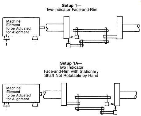
FIG. 3. Two-indicator face-and-rim alignment method.
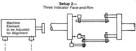
FIG. 4. Three-indicator face-and-rim alignment method.
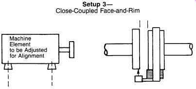
FIG. 5. Close-coupled face-and-rim alignment method.
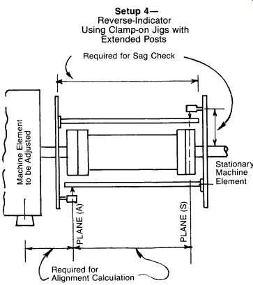
FIG. 6. Reverse-indicator alignment using clamp-on jigs.
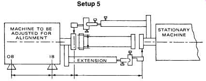
FIG. 7. Reverse-indicator alignment using face-mounted brackets or
any other brackets which hold the indicators as shown.
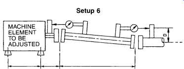
FIG. 8. Two-indicator face-face-distance alignment method
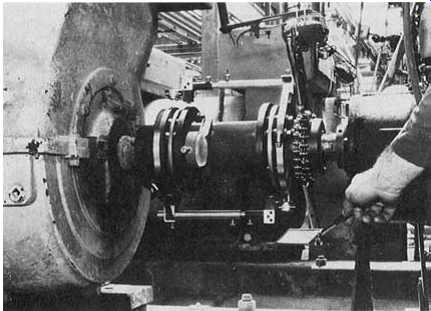
FIG. 9. Reverse-indicator setup.
1. Accuracy is not affected by axial movement of shafts in sleeve bearings.
2. Both shafts turn together, either coupled or with match marks, so coupling eccentricity and surface irregularities don’t reduce accuracy of alignment readings.
3. Face alignment, if desired, can be derived quite easily without direct measurement.
4. Rim measurements are easy to calibrate for bracket sag. Face sag, by contrast, is considerably more complex to measure.
5. Geometric accuracy is usually better with reverse-indicator method in process plants, where most couplings have spacers.
6. With suitable clamp-on jigs, the reverse-indicator method can be used quite easily for measuring without disconnecting the coupling or removing its spacer. This saves time, and for gear couplings, reduces the chance for lubricant contamination.
7. For the more complex alignment situations, where thermal growth and/or multi-element trains are involved, reverse-indicator can be used quite readily to draw graphical plots showing alignment conditions and moves. It’s also useful for calculating optimum moves of two or more machine elements, when physical limits don’t allow full correction to be made by moving a single element.
8. When used with jigs and posts, single-axis leveling is sufficient for ball-bearing machines, and two-axis leveling will suffice for sleeve bearing machines.
9. For long spans, adjustable clamp-on jigs are available for reverse indicator application, without requiring coupling spacer removal.
Face-and-rim jigs for long spans, by contrast, are usually non-adjustable custom brackets requiring spacer removal to permit face mounting.
10. With the reverse-indicator setup, we mount only one indicator per bracket, thus reducing sag as compared to face-and-rim, which mounts two indicators per bracket. (Face-and-rim can do it with one per bracket if we use two brackets, or if we remount indicators and rotate a second time, but this is more trouble.) There are some limitations of the reverse-indicator method. It should not be used on close-coupled installations, unless jigs can be attached behind the couplings to extend the span to 3 in. or more. Failure to observe this limitation will usually result in calculated moves which overcorrect for the misalignment.
Both coupled shafts must be rotatable, preferably by hand, and prefer ably while coupled together. If only one shaft can be rotated, or if neither can be rotated, the reverse-indicator method cannot be used.
If the coupling diameter exceeds available axial measurement span, geometric accuracy will be poorer with reverse-indicator than with face and-rim.
If required span exceeds jig span capability, either get a bigger jig or change to a different measurement setup such as face-face-distance.
Cooling tower drives would be an example of this.
Face-and-Rim Method
This is the "traditional" setup which is probably the most popular, although it’s losing favor as more people learn about reverse-indicator.
Advantages of face-and-rim:
1. It can be used on large, heavy machines whose shafts cannot be turned.
2. It has better geometric accuracy than reverse-indicator, for large diameter couplings with short spans.
3. It’s easier to apply on short-span and small machines than is reverse indicator, and will often give better accuracy.
Limitations of face-and-rim:
1. If used on a machine in which one or both shafts cannot be turned, some runout error may occur, due to shaft or coupling eccentricity.
2. If used on a sleeve bearing machine, axial float error may occur. One method of avoiding this is to bump the turned shaft against the axial stop each time before reading. Another way is to use a second face indicator 180° around from the first, and take half the algebraic difference of the two face readings after 180° rotation from zero start.
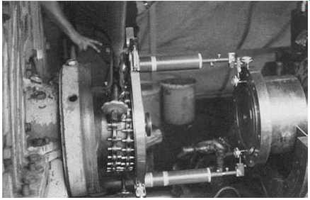
FIG. 10 illustrates this alignment method. Two 2-in. tubular graphite
jigs are used for light weight and high rigidity.
3. If used with jigs and posts, two or three axis leveling is required, for ball and sleeve bearing machines respectively. Reverse-indicator requires leveling in one less axis for each.
4. Face-and-rim has lower geometric accuracy than reverse-indicator, for spans exceeding coupling or jig diameter.
5. Face sag is often insignificant, but it can occur on some setups, and result in errors if not accounted for. Calibration for face sag is considerably more complex than for rim sag.
6. For long spans, face-and-rim jigs are usually custom-built brackets requiring spacer removal to permit face mounting. Long-span reverse-indicator jigs, by contrast, are available in adjustable clamp on models not requiring spacer removal.
7. Graphing the results of face-and-rim measurements is more complex than with reverse-indicator measurements.
Face-Face-Distance Method
Advantages of face-face-distance:
1. It’s usable on long spans, such as cooling tower drives, without elaborate long-span brackets or consideration of bracket sag.
2. It’s the basis for thermal growth measurement in the Indikon proximity probe system, and again is unaffected by long axial spans.
3. It’s sometimes a convenient method for use with diaphragm couplings such as Lucas Aerospace ( Utica, New York), allowing mounting of indicator holders on spacer tube, with indicator contact points on diaphragm covers.
FIG. 10. Face-and-rim indicator setup using lightweight, high-rigidity tubular graphite fiber-reinforced epoxy jigs.
Limitations of face-face-distance:
1. It has no advantage over the other methods for anything except long spans.
2. It cannot be used for installations where no coupling spacer is present.
3. Its geometric accuracy will normally be lower than either of the other two methods.
4. It may or may not be affected by axial shaft movement in sleeve bearings, but this can be avoided by the same techniques as for face-and rim.
Laser-Optic Alignment
In the early 1980s, by means of earth-bound laser beams and a reflector mounted on the moon, man has determined the distance between earth and the moon to within about 6 inches.
Such accuracy is a feature of optical measurement systems, as light travels through space in straight lines, and a bundled laser ray with particular precision.
Thus, critical machinery alignment, where accuracy of measurement is of paramount importance, is an ideal application for a laser-optic alignment system.
The inherent problems of mechanical procedure and sequence of measuring have been solved by Prüftechnik Dieter Busch, of Ismaning, Germany, whose OPTALIGN system ( FIG. 11) comprises a semi conductor laser emitting a beam in the infrared range (wavelength 820 mm), along with a beam finder incorporating an infrared detector. The laser beam is refracted through a prism and is caught by a receiver/detector.
These light-weight, nonbulky devices are mounted on the equipment shafts, and only a cord-connected microcomputer module is external to the beam emission and receiver/detector devices.
The prism redirects the beam and allows measurement of parallel offset in one plane and angularity in another, thus simultaneously controlling both. In one 90° rotation of the shafts all four directional alignment corrections are determined.
With the data automatically obtained from the receiver/detector, the microcomputer instantaneously yields the horizontal and vertical adjustment results for the alignment of the machine to be moved.
Physical contact between measuring points on both shafts is no longer required, as this is now bridged by the laser beam, eliminating the possibilities for error arising from gravitational hardware sag as well as from sticky dial indicators, etc. The system's basic attachment is still carried out with a standard quick-fit bracketing system, or with any other suitable attachment hardware.
If the reader owns an OPTALIGN® or the newer "smartALIGN" ( FIG. 12) system, he does not have to be concerned with sag. Other reader must continue the checkout process.
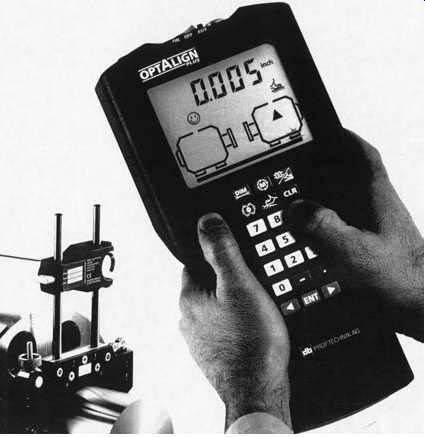
FIG. 11. Optalign laser-optic alignment system.
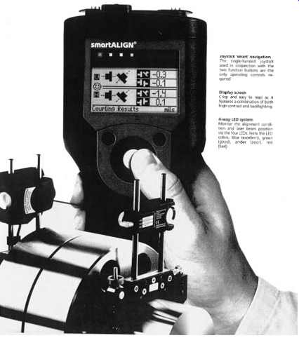
FIG. 12. SmartALIGN system. (Source: Prüftechnik, A. G., Ismaning,
Germany.)
Checking for Bracket Sag
Long spans between coupling halves may cause the dial indicator fixture to sag measurably because of the weight of the fixture and the dial indicators. Although sag may be minimized by proper bracing, sag effects should still be considered in vertical alignment. To determine sag, install the dial indicators on the alignment fixture in the same orientation and relative position as in the actual alignment procedure with the fixture resting on a level surface as shown in FIG. 13. With a small sling and scale, lift the indicator end of the fixture so that the fixture is in the horizontal position. Note the reading on the scale. Assume For example that the scale reading was 7.5 lbs. Next, mount the alignment fixture on the coupling hub with the dial indicator plunger touching the top vertical rim of the opposite coupling hub. Set the dial indicator to zero. Next, locate the sling in the same relative position as before and, while observing the scale, apply an upward force so as to repeat the previous scale reading (assumed 7.5 lbs in our example). Note the dial indicator reading while holding the upward force. Let us assume For example that we observe a dial indicator reading of -0.004 in. Using this specific methodology, sag error applies equally to the top and bottom readings. Therefore, the sag correction to the total indicator reading is double the indicated sag and must be algebraically subtracted from the bottom vertical parallel reading, i.e., -(2) (-0.004) =+0.008 correction to bottom reading.
This method is a clever one for face-mounted brackets. For clamp-on brackets, however, it would be easier and more common to attach them to a horizontal pipe on sawhorses, and roll top to bottom. FIG. 14 shows this conventional method which, except for the sag compensator device, is almost universally employed. The sag compensator feature incorporates a weight-beam scale which applies an upward force when the indicator bracket is located at the top of the machine shaft, and an equal, but opposite, force when the indicator bracket and shaft combination is rotated to the down position, 180° removed.
In any event, let us assume that we obtain readings of 0 and +0.160 in. at the top and bottom vertical parallels respectively. We correct for sag in the following manner:
FIG. 13. Testing for bracket sag.
FIG. 14. Sag compensator.
Using the first method of sag determination, we observe bottom parallel reading 0.160in.
Sag correction
Corrected bottom parallel reading
Bracket Sag Effect on Face Measurements
Bracket sag is generally thought to primarily affect rim readings, with little effect on face readings. Often this is true, but some risk may be incurred by assuming this without a test. Unlike rim sag, face sag effect depends not only on jig or bracket stiffness, but on its geometry.
Determining face sag effect is fairly easy. First get rim sag for span to be used (we are referring here to the full indicator deflection due to sag when the setup is rotated from top to bottom). This may be obtained by trial, with rim indicator only, or from a graph of sags compiled for the bracket to be used. Then install a setup with rim indicator only, on calibration pipe or on actual field machine, and "lay on" the face indicator and accessories, noting additional rim indicator deflection when this is done. Double this additional deflection, and add it to the rim sag found previously, if both the face and rim indicators are to be used simultaneously. If the face and the rim indicators are to be used separately, to reduce sag, use the original rim sag in the normal manner, and use this same original rim sag as shortly to be described in determining face sag effect-in this latter case utilizing a rim indicator installed temporarily with the face indicator for this purpose. If the face indicator is a different type (i.e., different weight) from the rim indicator, obtain rim sag using this face indicator on the rim, and use this figure to determine face sag effect.
Now install face and rim setup on the actual machine, and zero the indicators. With indicators at the top, deflect bracket upward an amount equal to the appropriate rim sag, reading on the rim indicator, and note the face indicator reading. The face sag correction with indicators at bottom would be this amount with opposite sign. If zeroing the setup at the bottom, the face sag correction at the top would be this amount with same sign (if originally determined at top, as described).
Face Sag Effect-Examples
Example 1
Face and rim indicators are to be used together as shown in FIG. 3. Assume you will obtain the following from your sag test:
Mount the setup on the machine in the field, and with indicators at top, deflect the bracket upward 0.007 in. as measured on the rim indicator.
When this is done, the face indicator reads plus 0.002 in. Face sag correction at the bottom position would therefore be minus 0.002 in. If you wish to zero at the bottom for alignment, but otherwise have data as noted, the face sag correction at the top would be plus 0.002 in.
Example 2
Face and rim indicators are to be used separately to reduce sag. Both indicators are the same type and weight. Other basic data are also the same.
Install face indicator and temporary rim indicator on the machine in the field, and place in top position. Zero indicators and deflect upward 0.004 in. as measured on rim indicator. Face indicator reads plus 0.0013 in. Face sag correction at the bottom would therefore be minus 0.0013 in. If zeroing at the bottom for alignment, but otherwise the same as above, face sag correction at top would be plus 0.0013 in.
Rim sag with rim indicator only Rim sag with two indicators
Example 3
This will determine sag for "3-Indicator Face-and-Rim Setup" shown in FIG. 4.
Set up the jig to the same geometry as for field installation but with rim indicator only and roll 180° top to bottom on pipe to get total single indicator rim sag ____ (Step 1).
Zero rim indicator on top and add or "lay on" face indicator, noting rim indicator deflection that occurs ____ (Step 2). Double this ____ (Step 3).
Add it to original total single indicator rim sag (Step 1). ____ (Step 4).
This figure, preceded by a plus sign, will be the sag correction for the rim indicator readings taken at bottom.
With field measurement setup as shown, zero all indicators, and deflect the indicator end of the upper bracket upward an amount equal to the total rim sag (Step 4). Note the face sag effect by reading the face indicator.
This amount, with opposite sign, is the face sag correction to apply to the readings taken at the lower position ____ (Step 5).
Now deflect the upper bracket back down from its "total rim sag" deflection an amount equal to Step 3.
The amount of sag remaining on the face indicator, preceded by the same sign, is the sag correction for the single face indicator being read at the top position ____ (Step 6).
All of the foregoing refers of course to bracket sag. In long machines, we will also have shaft sag. This is mentioned only in passing, since there is no need to do anything about it at this time. Our "point-by-point" alignment will automatically take care of shaft sag. For initial leveling of large turbo-generators, etc., especially if using precision optical equipment, shaft sag must be considered. Manufacturers of such machines know this, and provide their erectors with suitable data for sag compensation. Further discussion of shaft sag is beyond the scope of this text.
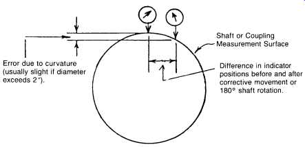
FIG. 15. Error can be induced due to curvature effect on misaligned
components.
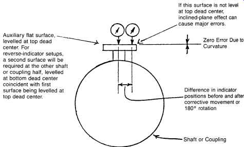
FIG. 16. Auxiliary flat surface added to avoid curvature-induced measurement
error.
Leveling Curved Surfaces
It’s common practice to set up the "rim" dial indicators so their contact tips rest directly on the surface of coupling rims or shafts. If gross mis alignment is not present, and if coupling and/or shaft diameters are large, which is usually the case, accuracy will often be adequate. If, however, major misalignment exists, and/or the rim or shaft diameters are small, a significant error is likely to be present. It occurs due to the measurement surface curvature, as illustrated in Figures 15 and 16.
This error can usually be recognized by repeated failure of top-plus bottom (T + B) readings to equal side-plus-side (S + S) readings within one or two thousandths of an inch, and by calculated corrections resulting in an improvement which undershoots or overshoots and requires repeated corrections to achieve desired tolerance. A way to minimize this error is to use jigs, posts, and accessories which "square the circle." Here we attach flat surfaces or posts to the curved surfaces, and level them at top and bottom dead center. This corrects the error as shown in FIG. 14.
For this method to be fully effective, rotation should be performed at accurate 90° quadrants, using inclinometer or bubble-vial device.
In most cases, however, this error is not enough to bother eliminating- it’s easier just to make a few more corrective moves, reducing the error each time.
Jig Posts
The preceding explanation showed a rudimentary auxiliary surface, or "jig post," used for "squaring the circle." A more common reason for using jig posts is to permit measurement without removing the spacer on a concealed hub gear coupling. If jig posts are used, it’s important that they be used properly. In effect, we must ensure that the surfaces contacted by the indicators meet these criteria:
• As already shown, they must be leveled in coordination at top and bottom dead centers, to avoid inclined plane error
• If any axial shaft movement can occur, as with sleeve bearings, the surfaces should also be made parallel to their shafts. This can be done by leveling axially at the top, rotating to the bottom, and rechecking.
If bubble is not still level, tilt the surface back toward level for a half correction.
• If face readings are to be taken on posts, the post face surfaces should be machined perpendicular to their rim surfaces. In addition to this, and to Steps 1 and 2 just described, rotate shafts so posts are horizontal. Using a level, adjust face surfaces so they are vertical. Rotate 180° and recheck with level. If not still vertical, tilt back toward vertical to make a half correction on the bubble. This will accomplish our desired objective of getting the face surface perpendicular to the shaft in all measurement planes.
The foregoing assumes use of tri-axially adjustable jig posts. If such posts are not available, it may be possible to get good results using accurately machined nonadjustable posts. If readings and corrections don’t turn out as desired, however, it could pay to make the level checks as described-they might pinpoint the problem and suggest a solution such as using a non-post measurement setup.
Interpretation and Data Recording
Due to sag as well as geometry of the machine installation, it’s difficult and deceptive to try second-guessing the adequacy of alignment solely from the "raw" indicator readings. It’s necessary to correct for sag, then note the "interpreted" readings, then plot or calculate these to see the overall picture-including equivalent face misalignment if primary readings were reverse-indicator on rims only. Sometimes thermal offsets must be included, which further complicates the overall picture.
As a way to systematically consider these factors and arrive at a solution, it’s helpful to use prepared data forms and stepwise calculation.
Suppose we are using the two-indicator face-rim method shown in FIG. 3; let's call it "Setup #1." To start, prepare a data sheet as shown in FIG. 17. Next, measure and fill in the "basic dimensions" at the top.
Then, fill in the orientation direction, which is north in our example. Next, take a series of readings, zeroing at the top, and returning for final readings which should also be zero or nearly so. Now do a further check: Add the top and bottom readings algebraically (T + B), and add the side readings (S + S). The two sums should be equal, or nearly so. If the checks are poor, take a new set of readings. Do the checks before accounting for bracket sag. Now, fill in the known or assumed bracket sag. If the bracket does not sag (optimist!), fill in zero. Combine the sag algebraically with the vertical rim reading as shown, and get the net reading using (+) or (-) as appropriate to accomplish the sag correction. A well-prepared form will have this sign printed on it. If it does not, mentally figure out what must be done to "un-sag" the bracket in the final position, and what sign would apply when doing so.
Now we are ready to interpret our data in the space provided on the form. To do this, first take half of our net rim reading:
This is because we are looking for centerline rather than rim offset.
Since its sign is minus, we can see from the indicator arrangement sketch that the machine element to be adjusted is higher than the stationary element, at the plane of measurement. This assumes the use of a conventional American dial indicator, in which a positive reading indicates contact point movement into the indicator.
By the same reasoning, we can see that the bottom face distance is 0.007 in. wider than the top face distance.
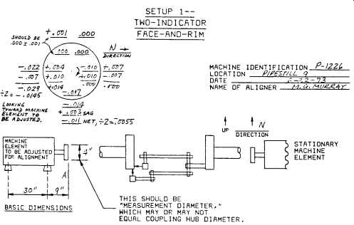
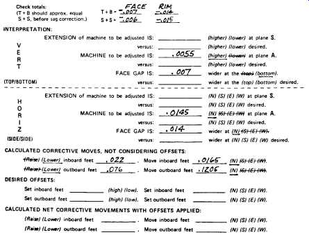
FIG. 17. Basic data sheet for two-indicator face-and-rim method.
Going now to the horizontal readings, we make the north rim reading zero by adding -0.007 in. to it. To preserve the equality of our algebra, we also add -0.007 in. to the south rim reading, giving us -0.029 in. Taking half of this, we find that the machine element to be adjusted is 0.0145 in. north of the stationary element at the plane of measurement.
Finally, we do a similar operation on our horizontal face readings, and determine that the north face distance is wider by 0.014 in.
The remaining part of the form provides space to put the calculated corrective movements. Although these have been filled in for our example, let's leave them for the time being, since we are not yet ready to explain the calculation procedure. We will show you how to get these numbers later. If you think you already know how, go ahead and try-the results may be interesting.
You have now seen the general idea about data recording and interpretation. By doing it systematically, on a prepared form corresponding to the actual field setup, you can minimize errors. If you are interrupted, you won’t have to wonder what those numbers meant that you wrote down on the back of an envelope an hour ago. We will defer consideration of the remaining setups, until we have explained how to calculate alignment corrective movements. We will then take numerical examples for all the setups illustrated, and go through them all the way.
Calculating the Corrective Movements
Many machinists make alignment corrective movements by trial and error. A conscientious person can easily spend two days aligning a machine this way, but by knowing how to calculate the corrections, the time can be cut to two hours or less.
Several methods, both manual and electronic, exist for doing such calculations. All, of course, are based on geometry, and some are rather complicated and difficult to follow. For those interested in such things, see References 1-15. Years ago, the alignment specialist made use of programmable calculator solutions. Perhaps he used popular calculators such as the TI 59 and HP 67. By recording the alignment measurements on a prepared form, and entering these figures in the prescribed manner into the calculator, the required moves came out as answers. A variation of this was the TRS 80 pocket computer which had been programmed to do alignment calculations via successive instructions to the user telling him what information to enter.
By far the simplest calculator is the one described earlier in conjunction with the laser-based OPTALIGN and smartALIGN systems.
The foregoing electronic systems are popular, and have advantages in speed, accuracy, and ease of use. They have disadvantages in cost, usability under adverse field and hazardous area conditions, pilferage, sensitivity to damage from temperature extremes and rough handling, and availability to the field machinist at 2:00 A.M. on a holiday weekend. They also, for the most part, work mainly with numbers, and the answers may require acceptance on blind faith. By contrast, graphical methods inherently aid visualization by showing the relationship of adjacent shaft centerlines to scale.
Manual calculation methods have the advantage of low investment (pencil and paper will suffice, but even the simplest calculator will be faster). They have the disadvantage, some say, of requiring more thinking than the programmed electronic solutions, particularly to choose the plus and minus signs correctly.
The graphical methods, which "old-timers" prefer, have the advantage of aiding visualization and avoiding confusion. Their accuracy will some times be less than that of the "pure" mathematical methods, but usually not enough to matter. Investment is low-graph paper and plotting boards are inexpensive. Speed is high once proficiency is attained, which usually does not take long.
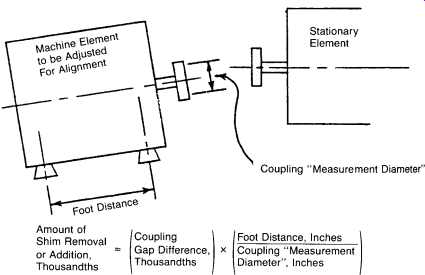
FIG. 18. Basic mathematical formula used in determining alignment corrections.
In this text, we will emphasize the graphical approach. Before doing so, let's highlight some common manual mathematical calculations.
Nelson published an explanation of one rather simple method a number of years ago. A shortened explanation is given in FIG. 18. For our given example, this would work out as follows:
Gap difference: 0.007 in.
Foot distance: 30 in.
Coupling measurement diameter: 4 in.
Then, using rim measurements, determine parallel correction, and add or remove shims equally at all feet. Now do horizontal alignment similarly, and repeat as necessary.
Nelson's method is easy to understand, and it works. It’s basically a four-step procedure in this order:
1. Vertical angular correction.
2. Vertical parallel correction.
3. Horizontal angular correction.
4. Horizontal parallel correction.
It has three disadvantages, however. First, it requires four steps, whereas the more complex mathematical methods can combine angular and parallel data, resulting in a two-step correction. Secondly, it’s quite likely that initial angular correction will subsequently have to be partially "un-done," when making the corresponding parallel correction. Nobody likes to cut and install shims, then end up removing half of them. Finally, it’s designed only for face-and-rim setups, and does not apply to the increasingly popular reverse-indicator technique.
We will now show two additional examples, wherein the angular and parallel correction are calculated at the same time, for an overall two step correction. Frankly, we ourselves no longer use these methods, nor do we still use Nelson's method, but are including them here for the sake of completeness. Graphical methods, as shown later, are easier and faster.
In particular, the alignment plotting board should be judged extremely useful. Readers who are not interested in the mathematical method may wish to skip to our later page, where the much easier graphical methods are explained. But, in any event, here is the full mathematical treatment.
In our first example, we will reuse the data already given in our setup No. 1 data sheet.
First, we will solve for vertical corrections:
=- in say in shim addition beneath inboard feet, or removal beneath outboard feet, or a combination of the two, for a total of 0.053in. correction.
Using Nelson's method, we found it necessary to make a 0.053 in. shim correction. Let us arbitrarily say this will be a shim addition beneath the inboard feet. At the coupling face, we then get a rise of:
Since we were already 0.0055 in. too high here, this puts us too high. Therefore, subtract 0.0745 in. (call it 0.075 in.) at all feet. Thus our net shim change will be:
For the horizontal corrections, we proceed similarly:
Let us say the outboard feet move north 0.105 in. This makes the coupling face move south, pivoting about the inboard feet:
Since it was already 0.0145 in. too far north, it’s now:
too far south, as are the feet. Therefore, net correction will be:
It can be seen that our answers agree closely with those on the data sheet, which were obtained graphically. The differences are not large enough to cause us trouble in the actual field alignment correction.
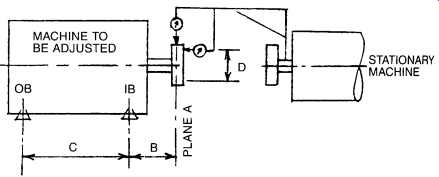
FIG. 19. Machine sketch for face-and-rim alignment method.
Move outboard feet 0.105in. + 0.017in. north; Move inboard feet 0.017in. north in; Outboard west feet must move north, inboard east feet must move south, or a combination of the two, for angular alignment.
Inboard in in feet: 0.053in. shim removal Outboard feet: 0.075in. shim removal
Alternatively, this first example could be solved with another similar "formula method." To begin with, we draw the machine sketch, FIG. 19. Then, we proceed by jotting down the relevant formulas:
For our example, the solutions would be as follows:
Vertical
As notice, the values found this way are close to those found earlier. The main problem people have with applying these formulas is choosing between plus and minus for the terms. The easiest way, in our opinion, is to visualize the "as found" conditions, and this will point the way that movement must proceed to go to zero misalignment. For example, our bottom face distance is wide-therefore we need to lower the feet (pivoting at plane A) which we denote with a minus sign. The machine element to be adjusted is higher at plane A-so we need to lower it some more, which takes another minus sign. For the horizontal, our north face distance is wider, so we need to move the feet north (again pivoting at plane A). The machine element to be adjusted is north at plane A, so we need to move it south. Call north plus or minus, so long as you call south the opposite sign. Not really hard, but a lot of people have trouble with the concept, which is why we prefer to concentrate on graphical methods, where direction of movement becomes more obvious.
We will get into this shortly, but first let's do a reverse-indicator problem mathematically.
For our reverse-indicator example, we will use the setup shown earlier as FIG. 6. Also, we must now refer to the appropriate data sheet, FIG. 20. Finally, we resort to some triangles, FIGS. 21 and 22, to assist us in visualizing the situation.
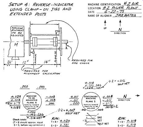
FIG. 20. Data sheet reverse-indicator alignment method.
FIG. 19 represents the elevation view. Solving, we obtain:
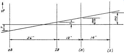
FIG. 21. Elevation triangles for reverse-indicator alignment example.
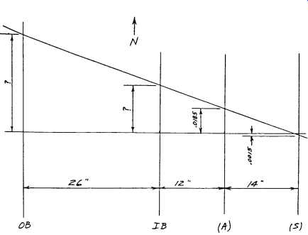
FIG. 22. Plan view triangles for reverse-indicator alignment example.
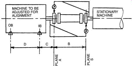
FIG. 23. Machine sketch for reverse-indicator alignment example.
Summarizing, we should:
Lower inboard feet 0.003 in.
Lower outboard feet 0.0065 in., say 0.007 in.
Move inboard feet south 0.036 in.
Move outboard feet south 0.073 in.
These results obviously agree closely with our graphical results. Again, the same results could have been obtained mathematically. To begin with, we have to provide a machine sketch, FIG. 23. Then:
Again, the answers come out all right if you get the signs right, but the visualization is difficult unless you make scale drawings or graphical plots representing the "as found" conditions.
The Graphical Procedure for Reverse Alignment
As mentioned earlier, the reverse dial indicator method of alignment is probably the most popular method of measurement, because the dial indicators are installed to measure the relative position of two shaft center lines. This section emphasizes this method because of the ease of graphically illustrating the shaft position.
What Is Reverse Alignment?
Reverse alignment is the measurement of the axis or the centerline of one shaft to the relative position of the axis of an opposing shaft center-line. This measurement can be projected the full length of both shafts for proper positioning if you need to allow for thermal movement. The measurement also shows the position of the shaft centerlines at the coupling
flex planes, for the purpose of selecting an allowable tolerance. The centerline measurements are taken in both horizontal and vertical planes ( FIG. 24).
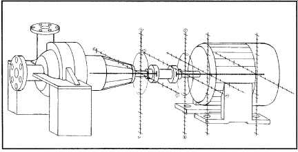
FIG. 24. Centerline measurement-both vertical and horizontal.
Learning How to Graph Plot
Graphical alignment is a technique that shows the relative position of the two shaft centerlines on a piece of square grid graph paper.
First we must view the equipment to be aligned in the same manner that appears on the graph plot. In this example we view the equipment with the "FIXED" on the left and the "MOVABLE" on the right ( Figure 5 25). This remains the same view both vertically and horizontally. Mark these sign conventions on graph paper, as shown in FIG. 26.
Example Scale: Each Square ´ = 1.0=
Scale: Each Square ; = 0.001=
Next, measure:
A. Distance between indicators B. Distance between indicator and front foot C. Distance between feet
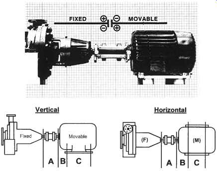 FIG. 25. Views of equipment to be aligned.
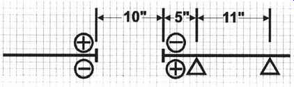
FIG. 26. Choose convenient sign convention on graph paper.
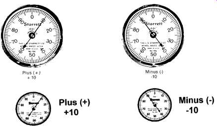
FIG. 27. Direction of indicator movements.
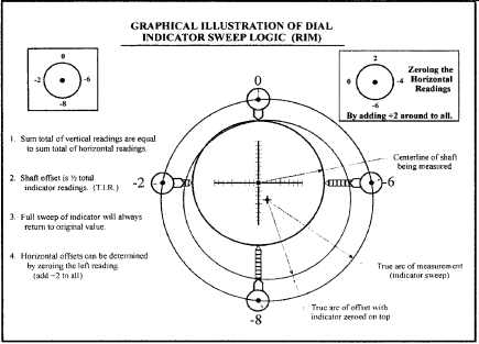
FIG. 28. Graphical illustration of dial indicator sweep logic. Measurements
are made on coupling rim.
The direction of indicator movements is shown in FIG. 27. Choose dial indicators that read 0.001-inch (or "one mil"), and become familiar with the logic of dial indicator sweeps ( FIG. 28). Note that this illustration shows the true arc of measurement. The centerline of the opposing shaft to be 0.004= lower and 0.002= to the right of the centerline of the shaft being measured.
The most important factors to remember about the logic of the dial indicator sweep are:
1. The plus and minus sign show direction.
2. The number value shows how far (distance).
3. The offset is 1/2 the total indicator reading (TIR).
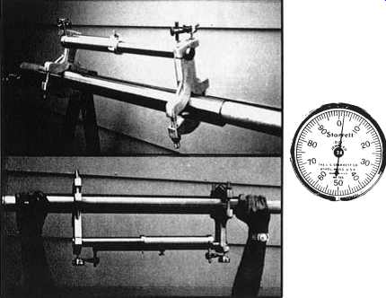
FIG. 29. Sag check. Example: 0.002= sag. Position indicator to read
+2.
Sag Check
To perform this check ( FIG. 29), clamp the brackets on a sturdy piece of pipe the same distance they will be when placed on the equipment. Zero both indicators on top, then rotate to bottom. The difference between the top and bottom reading is the sag.
Sag will always have a negative value, so when allowing for sag on the vertical move always start with a plus (+) reading.
Making the Moves
The next step is "making your moves," as illustrated in FIG. 30. The correct account of movement will have been predefined as discussed later in this segment.
Using the reverse method of centerline measurement, the tolerance window ( FIG. 31) can be visually illustrated on a piece of square grid graph paper. Each horizontal square will represent 1 inch, each vertical square will represent 1 one-thousandth of an inch (0.001=).
FIG. 31 shows a typical pump and motor arrangement with the coupling flex planes 8= apart. An allowable tolerance of 1/2 thousandths (0.0005=) per inch of coupling separation is selected. This is typical for equipment operating at speeds up to 10,000 rpm. The aligner will now apply the tolerance window to the graph paper 0.004= above and 0.004=below the fixed centerline at the same location where the flexing elements are shown in the figure.
After the adjustment has been made and a new set of indicator readings have been taken, if the movable centerline stays within the tolerance window at both flex planes, the alignment is now within tolerance.
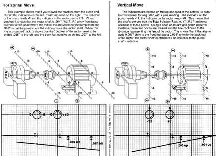
FIG. 30. Horizontal and vertical moves explained.
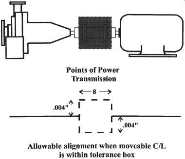
FIG. 31. Tolerance window ("tolerance box").
Thermal movement calculations need to be applied to ensure that the machine can move into tolerance and not move out of tolerance.
It should be noted that the generally accepted value is 1/2 thousandths per inch (0.0005=) deviation from colinear for each inch of distance between the coupling flex planes. This is probably too close a tolerance for general purpose pumps, but is not difficult to obtain. Since unwanted loads (thermal and other) are difficult to predict, the tighter tolerance gives a margin of safety.
Summary of Graphical Procedure
FIGS. 32 through 38 give a convenient summary of the graphical procedure.
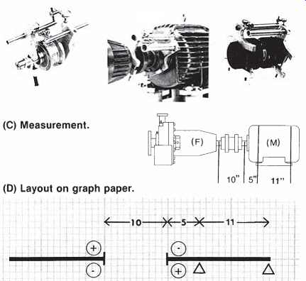
FIG. 32. Getting set up for the graphical procedure.
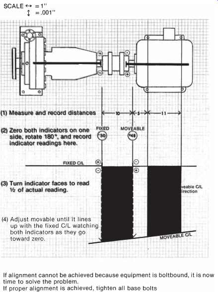
FIG. 33. Preliminary horizontal move.
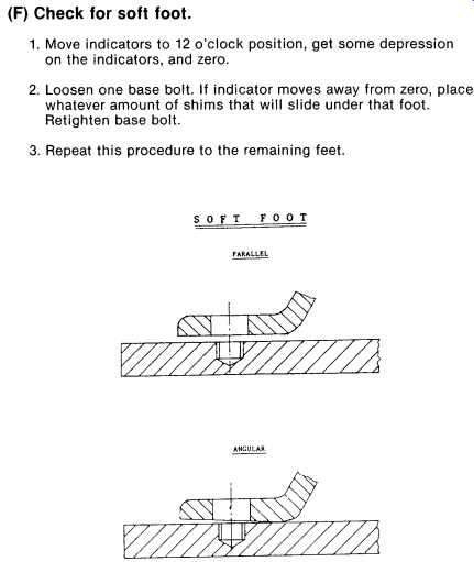
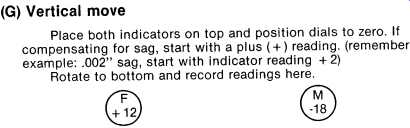
FIG. 34. Preparing for the vertical move includes soft foot check.
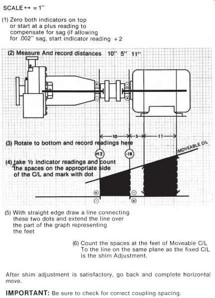
FIG. 35. Calculate the vertical move.
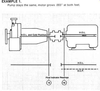
FIG. 36. Thermal growth considerations, parallel. Thermal movements
in machinery can be graphically illustrated when the aligner knows the
pre-calculated heat movements.
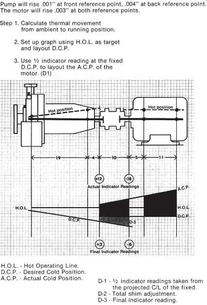
FIG. 37. Thermal growth considerations, angular.
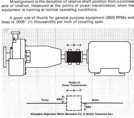
FIG. 38. Defining the "tolerance box."
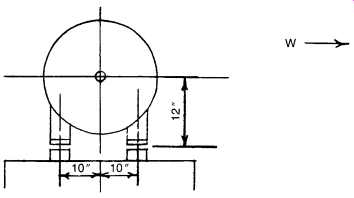
FIG. 39. Horizontal movement by vertical adjustment: electric motor
example.
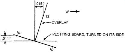
FIG. 40. Plotting board solution for electric motor movement exercise
of FIG. 39.
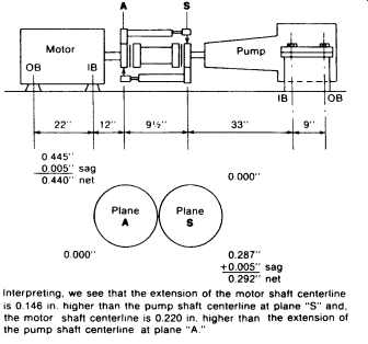
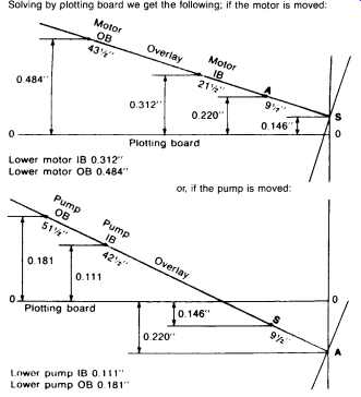
FIG. 41. Motor-pump vertical misalignment with single element move
solutions.
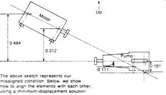
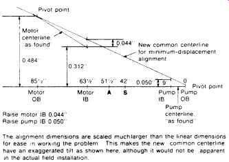
FIG. 42. Plotting board or graph paper plot showing optimum two-element
move.
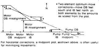
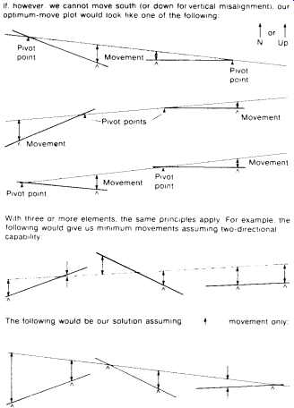
FIG. 43. Various possibilities in plotting minimum displacement alignment.
The "Optimum Move" Alignment Method
At times, as in mixing alcohol with water and measuring volumes, the whole can be less than the sum of its parts. A parallel situation exists in the method we are about to illustrate16. In effect, we will see that by making optimum movements of both elements to be aligned, the maximum movement required at any point is a great deal less than if either element were to be moved by itself. FIG. 39 shows an electric motor-driven centrifugal pump with severe vertical misalignment. The numbers are actual, from a typical job, and were not made up for purposes of this text.
As can be seen, regardless of whether we chose to align the motor to the pump or vice versa, we needed to lower the feet considerably-from 0.111 to 0.484 in. As it happened, the motor feet had only 0.025 in. total shimming, and the pump, as usual, had no shimming at all.
Some would shim the pump "straight up" to get it higher than the motor, and then raise the motor as required. This, in fact, was first attempted by our machinists. They had raised the pump about 3/8 in., at which point the piping interfered, and the pump was still not high enough. By inspection of FIGS. 41 and 5-42 it can be seen that they would have needed to raise it 0.484 in. (or 0.459 in. if all outboard motor shims had been removed).
FIG. 42 shows the solution used to achieve alignment without radical shimming or milling. As can be seen, our maximum shim addition was 0.050 in., which is much lower than the values found earlier for single-element moves. We could have reduced this shimming slightly by removing our 0.025 in. existing shims from beneath the outboard feet of the motor, but chose not to do so, leaving some margin for single element trim adjustments. As it turned out, the trimming went the other way, with 0.012 in. and 0.014 in. additions required beneath the motor inboard and outboard, respectively. This reflects such factors as heel and-toe effect causing variation in foot pivot centers. This is normal for situations such as this with short foot centers and long projections to measurement planes.
Several variations on the foregoing example are worth noting, and are shown in FIG. 43. The basic approach is the same for all though, and is easy to apply once the principle is understood.
We have, to this point, made no mention of thermal growth. If this is to be considered, the growth data may be superimposed on the basic mis alignment plots, or included prior to plotting, before proceeding with the optimum-move solution. Also, of course, there are valid non-graphical methods of handling the alignment solutions shown here-but we find the graphical approach easier for visualization, and accurate enough if done carefully.
Thermal Growth-Twelve Ways to Correct for It
Thermal growth of machines may or may not be significant for alignment purposes. In addition, movement due to pipe effects, hydraulic forces and torque reactions may enter the picture. Relative growth of the two or more elements is what concerns us, not absolute growth referenced to a
fixed benchmark (although the latter could have an indirect effect if piping forces are thereby caused). Vibration, as measured by seismic or proximity probe instrumentation, can give an indication of whether thermal growth is causing misalignment problems due to differences between ambient and operating temperatures. If no problem exists, then a "zero zero" ambient alignment should be sufficient. Our experience has been that such zero-zero alignment is indeed adequate for the majority of electric motor driven pumps. Zero-zero has the further advantage of simplicity, and of being the best starting point when direction of growth is unknown. Piping is often the "tail that wags the dog," causing growth in directions that defy prediction. For these reasons, we favor zero-zero unless we have other data that appear more trustworthy, or unless we are truly dealing with a predictable hot pump thermal expansion situation.
If due to vibration or other reasons it’s decided that thermal growth correction should be applied, several approaches are available, as follows:
1. Pure guesswork, or guesswork based on experience.
2. Trial-and-error.
3. Manufacturers' recommendations.
4. Calculations based on measured or assumed metal temperatures, machine dimensions, and handbook coefficient of thermal expansion.
5. Calculations based on "rules-of-thumb," which incorporate the basic data of 4.
6. Shut down, disconnect coupling, and measure before machines cool down.
7. Same as 6, except use clamp-on jigs to get faster measurements without having to break the coupling.
8. Make mechanical measurements of machine housing growth during operation, referenced to baseplate or foundation, or between machine elements. (Essinger.)
9. Same as 8, except use eddy current shaft proximity probes as the measuring elements, with electronic indication and/or recording.
10. Measure the growth using precise optical instrumentation.
11. Make machine and/or piping adjustments while running, using vibration as the primary reference.
12. Laser measurement represents another possibility. The OPTA LIGN method mentioned earlier also covers hot alignment checks.
Let us now examine the listed techniques individually.
Guesswork. Guesswork is rarely reliable. Guesswork based on experience, however, may be quite all right-although perhaps in such cases it isn't really guesswork. If a certain thermal growth correction has been found satisfactory for a given machine, often the same correction will work for a similar machine in similar service.
Trial-and-Error. Highly satisfactory, if you have plenty of time to experiment and don't damage anything while doing so. Otherwise, to be avoided.
Manufacturers' Recommendations. Variable. Some will work well, others will not. Climatic, piping, and process service differences can, at times, change the growth considerably from manufacturers' predictions based on their earlier average experience.
Calculations Based on Measured or Assumed Metal Temperatures, Machine Dimensions, and Handbook Coefficients of Thermal Expansion. Again, results are variable. An infrared thermometer is a useful tool here, for scanning a machine for temperature. This method ignores effects due to hydraulic forces, torque reactions, and piping forces.
Calculations Based on Rules of Thumb. Same comment as previous paragraph.
Shut Down, Disconnect Coupling, and Measure before Machines Cool Down.
About all this can be expected to do is give an indication of the credulity of the person who orders it done. In the time required to get a set of measurements by this method, most of the thermal growth and all of the torque and hydraulic effect will have vanished.
Same as Previous Paragraph Except Use Clamp-On Jigs to Get Faster Measurements Without Having to Break the Coupling. This method, used in combination with backward graphing, should give better results than 6, but how much better is questionable. Even with "quick" jigs, a major part of the growth will be lost. Furthermore, shrinkage will be occurring during the measurement, leading to inconsistencies. Measurement of torque and hydraulic effects will also be absent by this method. Some training courses advocate this technique, but we do not. If used, however, three sets of data should be taken, at close time intervals-not two sets as some texts recommend. The cooling, hence shrinkage, occurs at a variable rate, and three points are required to establish a curve for backward graphing.
Make Mechanical Measurements of Machine Housing Growth During Operation, Referenced to Baseplate or Foundation, or Between Machine Elements. This method can be used for machines with any type of coupling, including continuous-lube. Essinger describes one variation, using base plate or foundation reference points, and measurement between these and bearing housing via a long stroke indicator having Invar 36 extensions subject to minimum expansion-contraction error. Hot and cold data are taken, and a simple graphic triangulation method gives vertical and horizontal growth at each plane of measurement. This method is easy to use, where physical obstructions don’t prevent its use. Bear in mind that base plate thermal distortion may affect results. It’s reasonably accurate, except for some machines on long, elevated foundations, where errors can occur due to unequal growth along the foundation length. In such cases, it may be possible to apply Essinger's method between machine cases, without using foundation reference points. A further variation is to fabricate brackets between machine housings and use a reverse-indicator setup, except that dial calipers may be better than regular dial indicators which would be bothered by vibration and bumping.
Same as Previous Paragraph, But Use Eddy Current Shaft Proximity Probes as the Measuring Elements, with Electronic Indicating and/or Recording.
Excepting the PERMALIGN method, this one lends itself the best to keeping a continuous record of machine growth from startup to stabilized operation. Due to the complexity and cost of the instrumentation and its application, this technique is usually reserved for the larger, more complex machinery trains. Judging by published data, the method gives good results, but it’s not the sort of thing that the average mechanic could be fully responsible for, nor would it normally be justified for an average, two-element machinery train. In some cases, high machine temperatures can prevent the use of this method. The Dodd bars offer the advantage over the Jackson method that cooled posts are not needed and thermal distortion of base plate does not affect results. The Indikon system also has these advantages, and in addition can be used on unlimited axial spans. It is, however, more difficult to retrofit to an existing machine.
Measure the Growth Using Precise Optical Instrumentation. This method makes use of the precise tilting level and jig transit, with optical micrometer and various accessories. By referencing measurements to fixed elevations or lines of sight, movement of machine housing points can be determined quite accurately, while the machine is running. As with the previous method, this system is sophisticated and expensive, with delicate equipment, and requires personnel more knowledgeable than the average mechanic. It’s therefore reserved primarily for the more complex machinery trains. It has given good results at times, but has also given erroneous or questionable data in other instances. The precise tilting level has additional use in soleplate and shaft leveling, which are not difficult to learn.
Several consultants offer optical alignment services. For the plant having only infrequent need for such work, it’s usually more practical to engage such a consultant than to attempt it oneself.
Make Machine and/or Piping Adjustments While Running, Using Vibration as the Primary Reference. Baumann and Tipping describe a number of horizontal onstream alignments, apparently made with success. Others are reluctant to try such adjustments for fear of movement control loss that could lead to damage. We have, however, frequently adjusted pipe sup ports and stabilizers to improve pump alignment and reduce vibration while the pump was running.
Laser Measurements
With the introduction of the modern, up-to-date PERMALIGN system, laser-based alignment verification has been extended to cover hot alignment checks. FIG. 44 illustrates how the PERMALIGN® is mounted onto both coupled machines to monitor alignment. The measurements are then taken when the monitor (shown mounted on the left hand machine) emits a laser beam, which is reflected by the prism mounted on the other machine (shown on the right). The reflected beam reenters the monitor and strikes a position detector inside. When either machine moves, the reflected beam moves as well, changing its position in the detector. This detector information is then processed so that the amount of machine movement is shown immediately in terms of 1/100 mm or mils in the display, located directly below the monitor lens. Besides displaying detector X and Y co-ordinates, the LCD also indicates system temperature and other operating information.
Thermal Growth Estimation by Rules of Thumb
We will now describe several "rules of thumb" for determining growth.
Frankly, we have little faith in any of them, but are including them here for the sake of completeness.
The following is for "foot-mounted horizontal, end suction centrifugal pumps driven by electric motors":
For liquids 200°F and below, set motor shaft at same height as pump shaft.
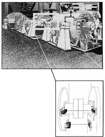
FIG. 44. Hot alignment of operating machines being verified by laser-optic
means (Prüftechnik A.G., Ismaning, Germany).
For liquids above 200°F, set pump shaft 0.001 in. lower, per 100°F of temperature above 200°F per in. distance between pump base and shaft centerline.
Example: 450°F liquid; pump dimension from base to centerline is 10 in.
The following applies to "foot mounted pumps or turbines:
Where L = Distance from base to shaft centerline, feet To = Operating temperature, °F Ta = Ambient temperature, °F For centerline mounted pumps, we are told to change the coefficient from 6 to 3. Another rule tells us to use the coefficient 3 for foot mounted pumps!
Yet another source tells us to use the following formula:
Another rule of thumb says to neglect thermal growth in centerline mounted pumps when fluid temperature is below 400°F, and to cool the pedestal when fluid temperature exceeds 400°F. This rule is somewhat unrealistic, since the benefits of omitting the cooling clearly outweigh the advantages of including it!
Yet another rule tells us to allow for 0.0015 in. growth per in. of height from base to shaft centerline, for any steam turbine-regardless of steam or ambient temperatures. Another chart goes into elaborate detail, recommending various differences in centerline height between turbine and pump based on machine types and service conditions, but without considering their dimensions.
Therma...
growth, inches,...
...centerline mounted pumps.
For foot mounted pumps, use L in place of ...
Therefore, set pump 0.025in. low
set motor 0.025in. high
For electric motor growth, we have the following:
(Foot to shaft centerline, in.) (6 x 10⁻⁶ ) (nameplate temp rise, °F) = motor vertical growth, in. This is inconvenient, since motor temperature rise is normally given in degrees centigrade. In case you have forgotten how to convert, °F = (°C x 9/5) + 32.
Another rule says to use half of the above figure.
Then there is the rule that advises using 7L, where L represents distance from base to shaft centerline in feet, and the answer comes out in thousandths of an inch. Yet another source says to use 4L. These rules all assume uniform vertical expansion from one end to the other. However, on motors having single end fans, the expansion will be greater at the air outlet end. Angular misalignment caused by this difference can exceed parallel misalignment caused by overall growth! The same can be true of certain other machines with a steep temperature gradient from one end to the other, such as blowers, compressors, and turbines.
The rules just cited were found in various published or filmed instructions from major pump manufacturers, oil refining companies and, in one case, a technical magazine published for the electric power industry. Their inconsistency, and their failure to recognize certain growth phenomena, make their accuracy rather questionable. This is especially true where piping growth can affect machine alignment.
Finally, the reader may wish to review either ref. 17 or 18, which give quick updates on shaft alignment technology.